Biogeographical research has long sought to document current and past species’ distributions through descriptive studies, but in recent decades this field has evolved to (1) capture local to coast-wide quantitative estimates of species’ abundances, (2) link physical processes with species’ distributions, and (3) determine how climate change disrupts biogeographic patterns. However, assessing change requires quantitatively robust data that are both geographically and temporally broad. Historically, such studies were rare, largely due to funding constraints. Here, we present a model for sustaining long-term, quantitative biogeography surveys using a collaborative approach. We also share some key contributions resulting from this model, including (1) a robust understanding of biogeographic patterns and the temporal dynamic of those patterns, (2) more comprehensive assessment of impacts at various scales (e.g., oil spill, coast-wide disease event), and (3) more informed management decisions (e.g., marine protected area design and evaluation).

> High res figure

Introduction

Understanding how physical processes shape patterns of species’ diversity and distribution over space and time has been a long-standing goal of biogeography (Dana, 1853; Lomolino et al., 2010). Traditionally, biogeographic studies tended to fall within one of two temporal extremes—ecological biogeography employed one-off, descriptive surveys designed to document extant species’ presence/absence (particularly to establish species’ range boundaries), while historical biogeography utilized phylogenetic and geological information to infer patterns of species’ relationships and distributions through geologic time (Jenkins and Ricklefs, 2011). These studies led to important discoveries about mechanisms that underlie broad biogeographic patterns (e.g., continental drift, major current patterns, climate and evolution; Sanford, 2013). In recent decades, marine ecologists have embraced the broad-scale approach used by biogeographers to identify the patterns and processes that drive species distributions (Jenkins and Ricklefs, 2011; Sanford, 2013; Witman et al., 2015). Climate change, with broadly reaching (large spatial, long temporal) but often unexpected impacts, was a major impetus for this shift, as was a need for predictive rather than reactionary information for policy and management. Accurate assessment of change requires broad-scale, quantitative, multi-decadal studies that allow for separation of natural variability in communities over space and time from true shifts in species’ distributions resulting from climate change (Mieszkowska et al., 2014).

The Partnership for Interdisciplinary Studies of Coastal Oceans (PISCO) was created in part as a model for the provision of informed and rigorous science essential for policymaking and policy managers. A core pillar of PISCO was to develop a long-term, spati‑ally extensive, feasible, and adequately funded program that would provide baseline data for assessing the structure and function of ecological communities. In order to both inform policy and assess natural and anthropogenic disturbances, we created:

1. A biogeographic network of monitoring sites to provide
   a. A baseline for judging patterns of change and dynamics of ecological communities
   b. Capacity for evaluation of questions of special interest (e.g., endangered species, disease, climate change, pollution impacts, fisheries management, coastal community resilience)
    
2. A query-enabled database
    
3. Web-based visualization tools available to the public, managers, policymakers, and other scientists
    
4. A diverse and buffered funding model, which is an essential component of any large-scale and long-term investigation

To attain our goals, we took a four-part approach:

1. We ran coastal biodiversity surveys (CBS) using two separate protocols to capture different aspects of biodiversity.
   a. A spatially nested protocol that allowed for characterization of spatial scaling of ecological communities.
   b. A geospatial grid protocol that employed fixed transects that run from high to low tidal zones to allow for three-dimensional mapping of species at each site and assessment of community change over time at local (vertical distribution) and geographic (latitudinal) scales.
    
2. We conducted long-term “key assemblage” surveys by designating fixed plots to target “key” species assemblages. “Key” species include foundation species (e.g., mussels) as well as those of special interest (e.g., sea stars, abalone). The plots are sampled annually for assessment of key species and community dynamics.
    
3. We instituted environmental monitoring.
    
4. We strictly enforced temporal stability of core methods to ensure data consistency.

PISCO focused on two major hard-bottom ecological systems in the coastal marine environment: shallow subtidal and intertidal habitats. A complementary large-scale oceanographic sampling program provided data used to understand the potential drivers of pattern and change.

Here, we report on the northeastern Pacific intertidal zone, one of the best-studied maritime systems in the world in terms of its population and community ecology (e.g., Paine, 1966; Connell, 1970; Menge, et al., 1994, 1997, 2004, 2015; Sagarin et al., 1999; Broitman et al., 2008), biogeography (e.g., Valentine, 1966; Murray and Littler, 1980; Blanchette et al., 2008), and phylogeography (e.g., Burton, 1998; Dawson, 2001, 2014; Wares et al., 2001; Pelc et al., 2009; Kelly and Palumbi, 2010). We describe key contributions produced by our unique collaborative effort, including: (1) scope of effort and assets, (2) spatial patterns detected, (3) temporal patterns detected, (4) mechanisms identified, (5) consequences, and (6) implications for policy and management.

 

Scope of Effort and Assets

Throughout PISCO’s history, the intertidal program has included many partners under an umbrella consortium called the Multi-Agency Rocky Intertidal Network, or MARINe (https://pacificrockyintertidal.org). The PISCO/MARINe collaboration is unusual in that it coordinates science, methods, policy, and funding, but especially prioritizes data coordination. Unexpectedly, this last function has had the greatest impact. Through development of standardized data entry protocols, a shared database with enforced rules and built-in quality assurance/quality control procedures, and a web-based information, data, and graphics production portal, PISCO/MARINe successfully brought into “data compliance” partners that could have produced separate and noncompatible programs. This core element—a common database—helped leverage a substantial and diverse funding portfolio. Increases in contributor numbers were based on recognition that their funds would add to and be matched by existing data assets. For example, if an effluent discharger was required to assess potential impacts of the effluent, they previously might have done a one-off assessment using discharge and reference sites. PISCO/MARINe offered an alternative: with an existing extensive PISCO/MARINe database and a standing research team, the discharger could fund PISCO/MARINe to conduct the study. The assessment would be based on consistent protocols, use either existing data or support collection of new data as appropriate, and would be rigorous and therefore easily defended. This approach decreases costs for all partners and greatly broadens the potential impact and usefulness of data assets.

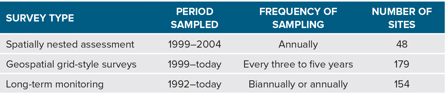
The scope of the program and data assets are summarized in Figure 1 and Table 1. Sampling occurs from the Gulf of California, Mexico, to Southeast Alaska, USA, and includes the entire California Current Large Marine Ecosystem (CCLME). The CBS spatially nested surveys occurred annually between 1999 and 2004 (48 sites sampled). Ongoing surveys include the CBS geospatial grid surveys begun 1999 (179 sites sampled every three to five years) and the long-term “key assemblage” program begun 1992 (154 sites sampled one to two times per year). We also maintain a coastal environmental sampling program for collecting geomorphological data (e.g., rock type, topography, rugosity, aspect, and slope) and temperature data (temperature loggers at 77 sites).

Detailed protocol information can be found in the literature (e.g., Schoch et al., 2006; Blanchette et al, 2008; Miner et al., 2018) and at our web portal (https://pacificrockyintertidal.org). Our website also shows our partners and describes program findings, provides data access, and has graphics capabilities that allow exploration of spatial and temporal patterns for over 300 species, physical attributes of sites (e.g., geology, rugosity, tidal exposure), and a suite of community metrics (e.g., measures of species diversity, stability, and vulnerability).

 

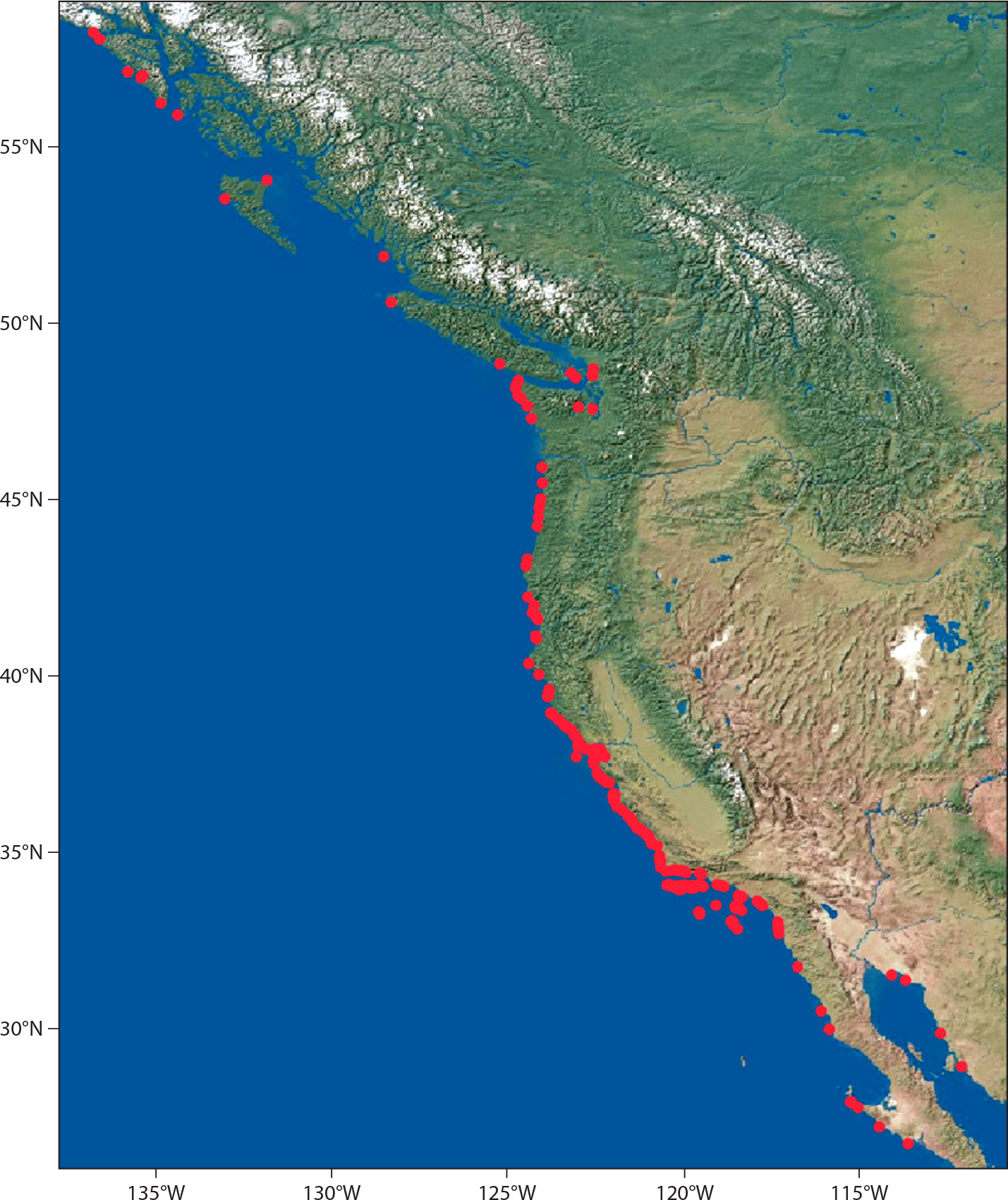
Figure 1. Spatial scope of biogeographic assessments. The map shows the 258 sites that have been sampled as part of the intertidal biogeographic assessment across the three main survey programs listed in Table 1. See the table for sites, number of years sampled, and frequency of sampling for each type. > High res figure

Table 1. Period sampled, frequency of sampling, and number of sites for each intertidal biogeographic program. > High res table

 

Key Findings

Below, we highlight some of the key contributions our monitoring program has made toward a better understanding of spatial and temporal biogeographic patterns along the west coast of North America, and how these findings have provided a basis for sound policy and management decisions. Boxes 1 and 2 summarize key messages.

 

Box 1. Key Lessons for Ecologists A biogeographic network of monitoring sites provides baseline data for assessing patterns of change and dynamics, and broad context for experimental and mechanistic studies. A consortium approach to monitoring, with standardized protocols and a centralized data repository, ensures data compatibility, fosters collaboration, and encourages a diverse funding portfolio. Biogeographic patterns of community similarity are highly correlated with sea surface temperature, but instrumentation for other key physical parameters that can be deployed on a broad scale need to be developed. Community level “climate velocity” might vary with latitude, which could have implications for scaling up from localized experiments.

 

Box 2. Key Lessons for Policymakers Knowing patterns of change and dynamics at broad scales (see Box 1) allows for more informed policy and management decisions. Long-term studies are essential for detecting and assessing impact (e.g., from non-native species invasion, disease events, climate change, oil spills, pollution) and for designing appropriate mitigation and recovery efforts. Marine disease events remain highly unpredictable in time and space. Broad-scale monitoring provides data necessary for building predictive models. Strong support of a monitoring consortium (through funding and/or direct participation) ensures data are: (1) appropriate for questions of interest, and (2) available for use via web display and data portals. Ability of communities to resist or recover from change might vary with latitude, and this should be considered when designating protection.

 

CBS: Spatially Nested Approach

Characteristic spatial scaling (Wiens, 1989) describes the spatial pattern of variance in some measured variable (e.g., density, community composition). Spatial scaling may be hierarchical, and each spatial scale in the community may reflect similar scaling of some ecological driver (see Edwards, 2004; Edwards and Estes, 2006). One efficient approach to assessment of characteristic spatial scaling relies on a spatially nested design (Edwards, 2004). This approach often uses variance components analysis to partition variance explained at each spatial scale. For example, Menge et al. (2015) quantified community structure across 13 sites spanning four capes in Oregon and northern California. They found that ~50% of the explained variance in community structure was associated with oceanic conditions and recruitment while ~25% could be linked to local-scale processes.

Understanding the processes that control species diversity at various scales has long been a goal of ecology (Witman et al., 2004). Schoch et al. (2006) designed a study to look for characteristic spatial scaling in biogeographic patterns and associated potential drivers of community composition using the CBS spatially nested data set. Sampling locations were selected using previously described major or minor biogeographic boundaries to divide the coastline between Cape Flattery, Washington, and San Diego, California, into six domains that each spanned hundreds of kilometers. Within each domain, areas with similar geography encompassing tens of kilometers were selected, and three sites were chosen on kilometer scales within each area. Finally, three segments measuring tens to hundreds of meters were selected within each site. Within each segment, community composition was measured by running a 50 m horizontal transect across the high (mean high high water), mid (mean sea level), and low (mean low low water) zones. Species composition and abundances were quantified along these transects within 10 randomly placed 50 × 50 cm quadrats.

Overall, Schoch et al. (2006) found that in the low zone, species richness was higher in the north at the segment, site, and area scales, but higher in the south at the domain scale. Trends may be driven by greater patchiness of macrophytes to the north, a pattern most likely to be picked up at smaller spatial scales. The reverse pattern seen at the largest scale is consistent with usual latitudinal diversity gradients and more reflective of the species pool from which smaller-scale sites draw for local-scale diversity patterns (Witman et al., 2004). No latitudinal richness trends occurred in the mid and high zones where macrophytes tend to be less abundant and less patchy.

Russell et al. (2006) used the spatially nested survey data set to investigate whether the relationship between regional species pools and local diversity varied with scale (Figure 2; also see Sanford, 2013, for a review of studies examining the effect of regional species pools). They found that prediction of local richness based on regional species pools breaks down at small spatial scales coincident with the spatial scaling of biological interactions; as spatial scales decrease, a given species should interact with an increasing fraction of included species, which should lead to an asymptotic relationship between the regional pool of species and richness at local scales (Figure 3; but see Cornell et al., 2007, for a counter-example).

 

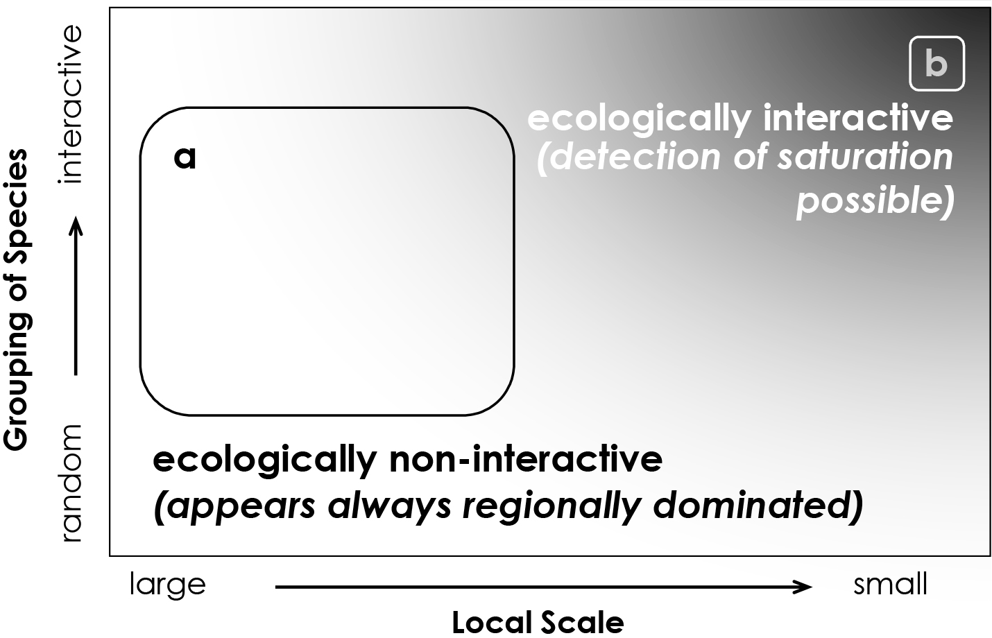
Figure 2. Model demonstrating spatial scale and species-grouping dependency of predictions from local-regional theory. (a) When “local” scales are large (relative to typical organismal size), ecologically heterogeneous areas or species are not interactive, and saturation is not expected. (b) When species groupings incorporate interacting species and local scales are small relative to typical organismal size, saturation is expected. Darker shading in this diagram signifies higher potential to detect community saturation. With permission from Russell et al. (2006). > High res figure

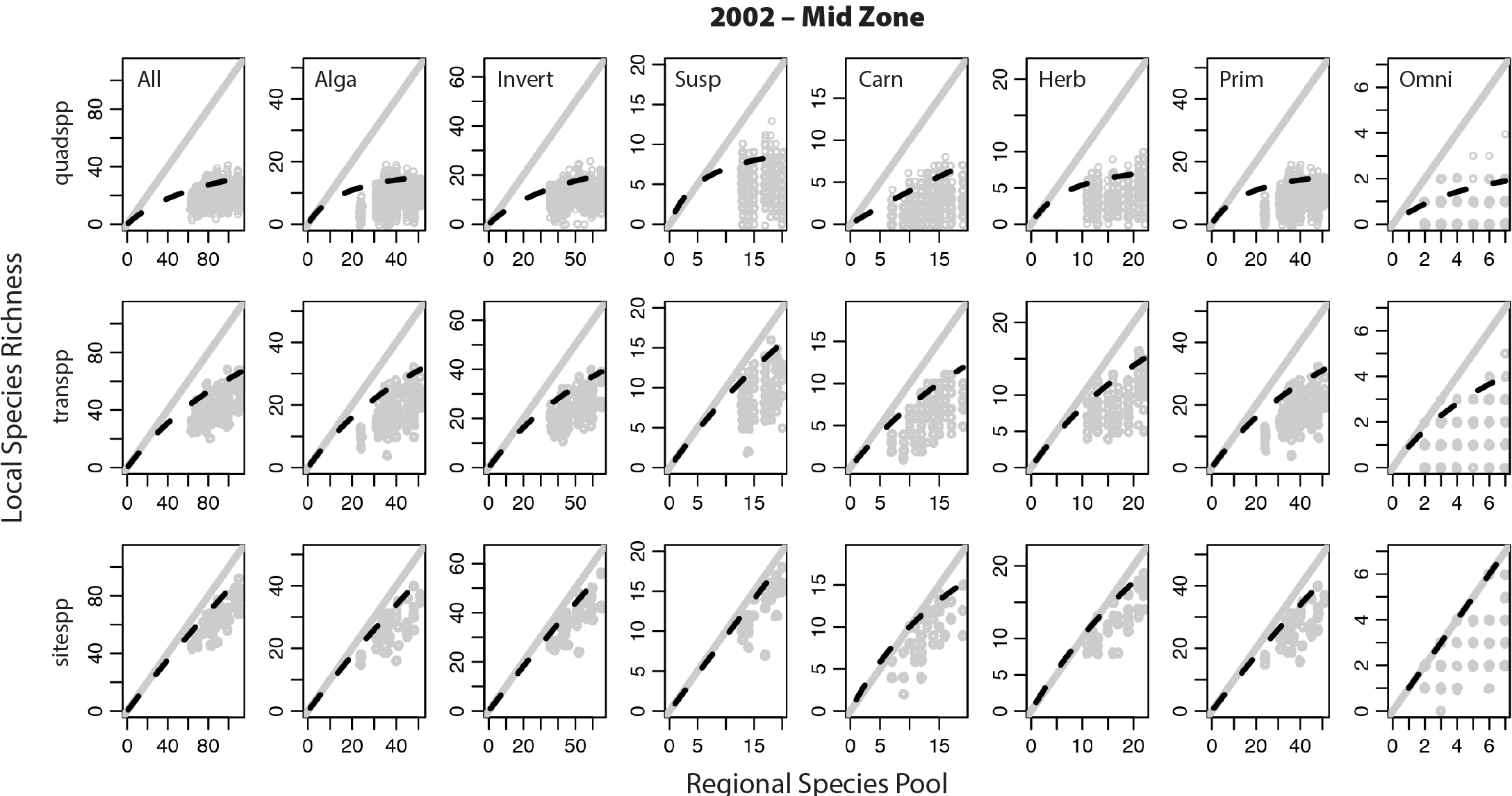
Figure 3. Relationship between local species richness and the regional species pool, where “local” is based on smaller (quadrat, top row) to larger (site, bottom row) spatial scales for rocky invertebrates and macrophytes. Gray dots are richness values at each spatial scale in annual surveys done from 2001 to 2004. Richness codes: All = all species. Alga = only algae. Invert = only invertebrates. Susp = suspension feeders only. Carn = carnivores only. Herb = herbivores only. Prim = all sessile organisms only. Omni = omnivorous species only. With permission from Russell (2005); see also Russell et al. (2006). > High res figure

 

Combining community survey data sets with modeling approaches can aid in detection of some aspects of dynamics. For example, Gouhier et al. (2010) found that fluctuations in mussel abundance vary between positive and negative synchronization, yielding a sine curve-like response at a scale of 600 km (e.g., Figure 4). Although such synchrony is often assumed to reflect environmental forcing, modeling suggested otherwise. Using meta-population models that assumed a dispersal distance of 100 km, disturbance-successional dynamic and predator-prey dynamic models recreated the synchronous pattern seen in nature. Specifically, the models showed that synchrony in population abundances was best explained by relatively limited dispersal distances interacting with local-scale species interactions.

 

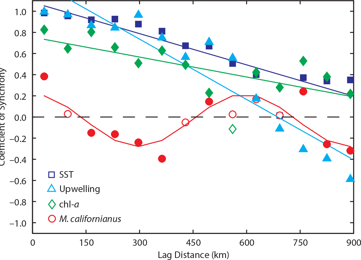
Figure 4. The dynamics of M. californianus cover and the environment along the US west coast. Spatial synchrony of the mean annual (1) M. californianus cover (red circles), sea surface temperature (SST; dark blue squares), chlorophyll-a (chl-a; green diamonds), and upwelling index (light blue triangles). The curves correspond to nonlinear (M. californianus) and linear (chl-a, SST, and upwelling index) statistical models fitted to each data set. Solid circles indicate statistical significance (α = 0.05). From Gouhier et al. (2010). > High res figure

 

CBS: Geospatial Grid Approach

Unlike the CBS spatially nested approach, sites sampled using the CBS geospatial approach were selected independently of spatial scaling. These surveys measured the abundance and distribution of all common taxa across the intertidal zone at fixed locations within the same set of sites, allowing for assessment of change in location of each taxon through time. At each site, a uniformly distributed grid was established, consisting of 11 vertical parallel transect lines spaced 3 m apart, with approximately 100 points per transect, each spanning the full tidal range. Organisms under each point were identified to the lowest possible taxonomic level, including layering and epibionts when appropriate (see https://www.pacificrockyintertidal.org). Mobile taxa were sampled within 50 × 50 cm quadrats placed randomly in the high, mid, and low zones along each transect, resulting in 33 total quadrats per grid. All sample points were georeferenced in three dimensions, allowing mapping of each community in three dimensions for assessment of spatial association patterns. Grid surveys also enabled tracking of vertical range shifts in species and community assemblages, potentially key metrics in assessment of climate-related change. CBS geospatial grid surveys are done at sites from Southeast Alaska to central Mexico, spanning several established biogeographic regions along the west coast of North America (Blanchette et al., 2008). As of spring 2019, this biodiversity database included data for over 700 taxa from 179 sites, most of which have been sampled multiple times.

With user-defined rules, the CBS geospatial grid approach can be used to identify geographic breaks in community structure. For example, a cluster analysis can be created in which sites are grouped based on community composition. The cluster pattern can then be used to describe geographic patterns. Especially with a large amount of data, cluster numbers partly depend on the differentiation threshold used, which often varies with the project goal. This method almost always leads to mismatches, sites grouping with others not in the same geographic area, which can lead to deeper exploration of the factors driving the clustering, such as local forcing.

Blanchette et al. (2008) used this approach to explore biogeographic patterns along the North American west coast. Using data for 296 taxa collected at 67 sites ranging from southern Alaska to northern Baja California Sur, Mexico, they identified 13 previously described biogeographic groupings as well as several “new” clusters. Although not formally tested, it was hypothesized that these previously unidentified groups might have resulted from localized features such as geology, upwelling, and wave exposure. After controlling for geographic distance, the spatial pattern of community similarity was highly correlated with long-term mean sea surface temperature as has been previously reported (Hubbs, 1948). This suggests that both geographical location and oceanographic forcing structure intertidal communities. Note that sea surface temperature is strongly associated with hydrographic conditions, which may affect other potential drivers of biogeography such as larval propagule dispersal (Watson et al., 2011; Castorani et al., 2015)

Fenberg et al. (2014) also utilized the CBS geospatial grid data set to assess whether biogeographic patterns could be explained by physical characteristics of the coastal environment. They used a random forest analysis to compare biogeographic patterns to 29 environmental factors. They found that the best predictors of community structure were nutrient concentrations, sea surface temperature, and upwelling, and that the associated explanatory variables varied by biogeographic region and species dispersal ability.

 

Spatiotemporal Patterns

Because whole-community biogeographic studies are costly, requiring a substantial level of participation by experts and, ideally, consistency of data collectors over time, assessment of temporal biogeographic dynamics is rare. However, for at least two reasons, the study of spatial patterns is much more valuable in a temporal framework. First, all ecological research is characterized by both signal and noise. What counts as signal or noise varies, but the goal is almost always to account for noise in order to detect signal. In biogeographic assessment, understanding of both noise and key spatiotemporal signals is in its infancy. For example, understanding the general static spatial biogeographic pattern (the signal) of a system is dependent on the random change in the pattern that will occur over time (the noise). Only after a period sufficient to “capture” and account for the underlying random noise in the system (which will vary system to system) will an unbiased and accurate assessment of the biogeographic pattern be possible.

A second and increasingly important reason for a temporal framework is the high likelihood that with climate change, environmental forcing will change biogeographic patterns in a nonrandom way (e.g., Sagarin et al., 1999; Parmesan and Yohe, 2003). This makes the signal-to-noise problem more difficult unless we have an estimate of the temporal pattern of change. For a static system, noise can be thought of as variance that obscures a value, which is possible to identify in multi­-
variate community composition space. However, challenges arise if the signal is a trend of unknown slope or if different community components have dissimilar slopes. Such trends could lead to unstable future species combinations. Hence static, one-time assessments are likely to become increasingly inaccurate, making temporal assessment critical.

Because of the programmatic features discussed above, the intertidal biogeographic monitoring program can and will continue to provide temporal assessment of biogeographic patterns and derived attributes such as geographic patterns of variation and directional velocity of change in ecological communities (sometimes termed climate velocity; Pinsky et al., 2013). This would not have been true in our program even five years ago because the signal-to-noise ratio was too low. That is, detection of significant change in ecological communities against a backdrop of multiple frequencies of environmental noise (e.g., random variation, El Niño-Southern Oscillation events, Pacific Decadal Oscillation) is difficult. (Note that for some assessments, “noise” might actually be the signal of interest.) Long-term, broad-scale monitoring programs are rare and challenging to sustain, but they are essential to understanding the temporal dynamics of biogeography. Below, we present recent examples of the understanding that can come from such temporal assessments.

 

Climate Change Impacts

Heightened concern about the potential effects of climate change on ecological communities led us to explore key questions relating to resilience of rocky intertidal communities, including whether the ability to resist or recover from a perturbation varies geographically. Such evaluations are data intensive because of the signal-to-noise problem discussed above. Details will be reported elsewhere, but the general findings are described here because they highlight the necessity for geographically broad, long-term data sets in detecting and forecasting community change.

First, we have found that community stability (measured as within-site temporal similarity of community) correlates with latitude: rocky intertidal communities at northern sites vary less than those at southern sites (author Miner, unpublished data). Second, we have explored climate velocity patterns for communities. Species climate velocity is the rate of change and direction in the centroid of a species’ distribution (Pinsky et al., 2006). By extension, climate velocity for community composition is the directional change rate in communities over time. Assessment of climate velocity at the community level is rarely possible (Walther, 2010; Doney et al., 2012) because it requires many species to be sampled at many sites, using identical methods, over many years. By design, these requirements are met by the CBS geospatial grid survey data. Initial results suggest that rocky intertidal community composition in the CCLME is shifting poleward (i.e., species composition at northern sites is transitioning toward that of southern sites) at an average rate of ~4 km per year (author Raimondi, unpublished data). Documenting shifts at the community level gives us a much deeper understanding of the impacts resulting from climate change because it incorporates how community interactions (e.g., competition, predation, facilitation) are affected by changing physical conditions, in combination with the responses of many individual species (Sanford, 2013).

 

Marine Disease

Long-term monitoring data spanning nearly the entire geographic range of the sea star Pisaster ochraceus allowed a comprehensive assessment of the impact of the recent (2014–present) wasting disease event. PISCO/MARINe scientists have reported on specific questions related to this event (Hewson et al., 2014; Menge et al., 2016; Miner et al., 2018; Moritsch et al., 2018), but here we provide a synthetic example that links the spatio­temporal assets of our intertidal program. Figure 5 summarizes the regional spatial and temporal results of time series data for sea surface temperature and sea star abundance (panel a), coast-wide observations of sea star wasting disease (panel b, largely from a PISCO/MARINe citizen science collaborative effort), and sea star size structure (panel c); note the pulse of recruits immediately after the wasting event. In many regions, sea stars were declining, and wasting symptoms were present before major temperature increases occurred (Figure 5a). The ability to link site-specific temperature and sea star abundances at a geographically broad scale was critical to evaluating patterns of disease emergence and putative mechanisms for wasting (Monica Moritsch, University of California, Santa Cruz, pers. comm., 2019), and it provides the population data necessary for assessing impact and potential for recovery (Miner et al., 2018). The linkage of these findings allows us to identify regions most at risk and begin to make predictions about when and where the next outbreak might occur.

 

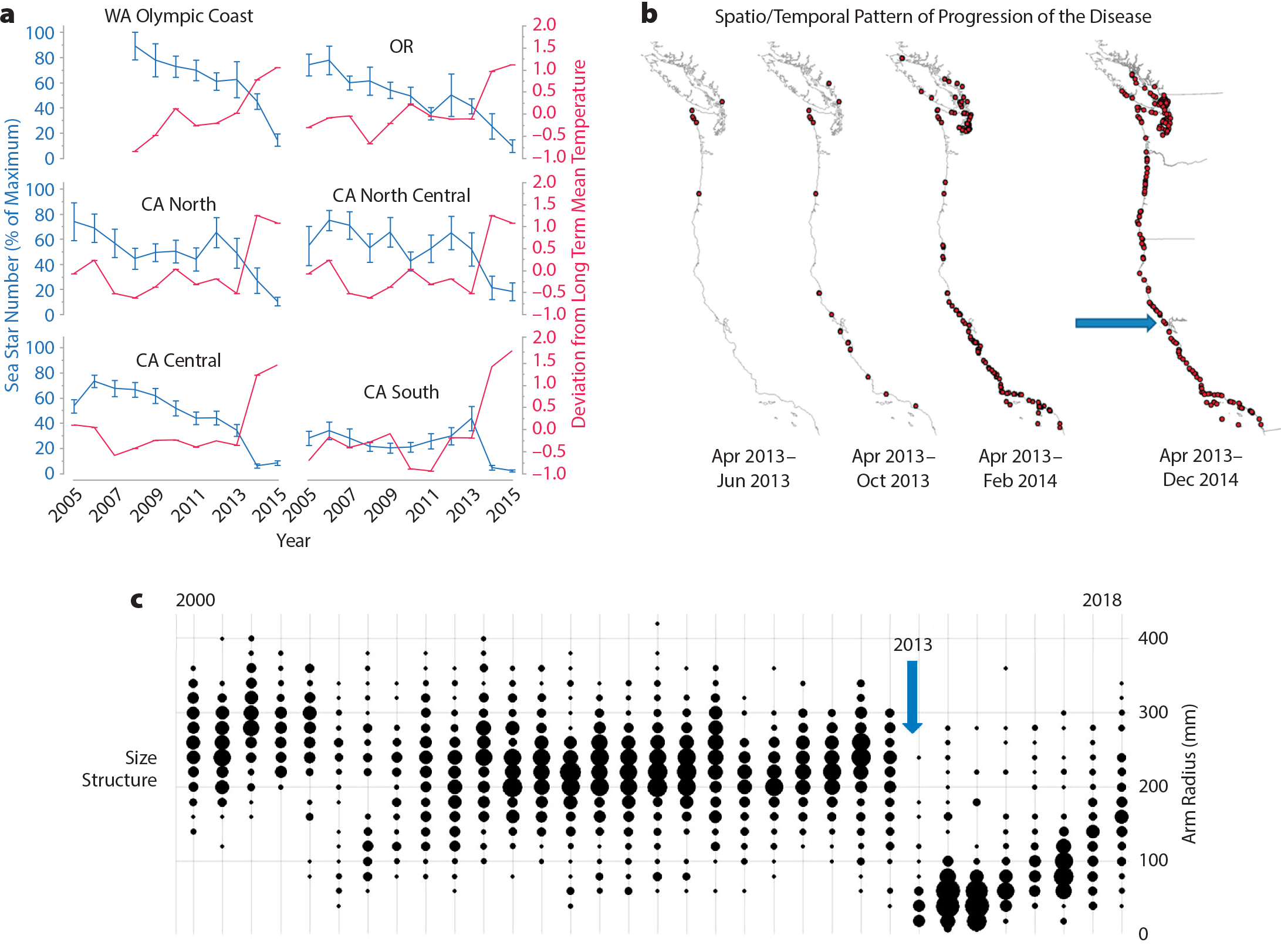
Figure 5. (a) General pattern of sea star (Pisaster ochraceus) abundance (relative to maximum) and average temperature (across all sampled sites) between 2000 and 2015. Each set of lines represents a different geographical region: the Olympic Coast of Washington, Oregon, Northern California, North Central California, Central California, and Southern California. (b) Spatiotemporal pattern of sea star wasting disease. The arrow indicates site location for data shown in panel c. (c) Size structure of P. ochraceus over time at a representative site. The vertical arrow indicates the year when wasting was first detected. Note that size structure was sampled twice per year between 2000 and 2015 and only once per year after 2015. Bubble size indicates the number of individuals of each size class. > High res figure

 

Assessments for the Implementation of Policy and Management

When developing the PISCO/MARINe intertidal biogeography program, we envisioned that our data and findings would be useful for policymakers and management more as contextual than integral information. In fact, we under­estimated the value of our data to policy and management. Over time, the core spatial and temporal survey designs, data collected, analytical results, and integrated assessments fundamentally altered policy implementation and resource management. In retrospect, this makes sense. In 1999, environmental policy was rapidly evolving toward an applied science valuing both social and “hard” science inputs. It was also a period of increasing understanding that environmental problems adhered to no formal boundaries or timeframes. Such changes in perspective led to an emerging appreciation of large-scale, long-term data sets. Policymakers and managers increasingly relied on them, leading to amplified support for their maintenance and, indeed, expansion. As noted above, this led to the possibility of a portfolio approach to funding.

The assets of the intertidal biogeographic program have been used in a number of applied projects. We briefly highlight two: (1) oil spill assessment, and (2) the design, initial characterization, and evaluation of marine protected areas (MPAs) in California and Oregon.

 

Oil Spills

One core source of funding for the intertidal biogeographic program has been the Bureau of Ocean Energy Management and its predecessor, the Minerals Management Service. As required by NOAA-based Natural Resources Damage Assessment, funding was based on needs for baseline and ongoing community assessments for use in case of oil spills. Two key assessment components are determination of loss and recovery trajectory. Over the last decade, there have been three major oil spills in the CCLME, two in San Francisco Bay (Cosco Busan in 2007, Raimondi et al., 2009; Dubai Star in 2009, Raimondi et al., 2011) and one near Santa Barbara (Refugio State Beach in 2015, Raimondi et al., 2019). For all three spills, our rocky intertidal data were used to assess impact and project recovery of the ecological communities affected. In addition, program data and analyses were used to determine compensatory mitigation in the form of habitat restoration. These efforts also highlight the rapid response capacity of the PISCO/MARINe intertidal program, as we were able to mobilize our expert field specialists within hours of the spills. This early work during the incidents was essential for Natural Resources Damage Assessment determinations.

 

Design, Initial Characterization, and Evaluation of Marine Protected Areas

The utility of the rocky intertidal bio­geography program to policy and management is perhaps best exemplified by its contribution to MPA implementation in California and, more recently, in Oregon. Data from the PISCO/MARINe biogeographic intertidal and subtidal databases were used to meet state-mandated requirements. MPAs are regions of coastline set aside to protect resources and/or habitat by limiting human activity within them. With the passage of the Marine Life Protection Act in 1999, California began the process of establishing what eventually became 124 MPAs protecting nearly 16% of state waters; 53 of these MPAs include intertidal habitat. Key charges of the MPA science advisory teams were to: (1) delineate biogeographic areas within regions to ensure protection across spatial scales, and (2) determine the minimum area required to adequately represent a given habitat and protect 90% of available species in the area. Following MPA establishment, a comprehensive multi-habitat monitoring program determined baseline conditions of MPAs and reference areas, and was used to assess the temporal pattern of community change and MPA effectiveness.

 

Discussion

Biogeography originated as a means of identifying patterns in species distributions and diversity, primarily from descriptive studies of presence/absence (Dana, 1853). Studies tended to investigate potential drivers of patterns at one of two temporal extremes: present-day conditions (primarily species range edges) or across geologic time. Present-day depictions were seminal in ecology because range edges often pointed to strong physical (e.g., currents, temperature, habitat) or biological (e.g., competition, predation, life history traits) drivers of species abundance (Blanchette et al., 2008; Lomolino et al., 2010; Sanford, 2013; Witman et al., 2015). Historical biogeography studies significantly advanced the fields of geology and evolutionary biology through the discovery or support of groundbreaking ideas such as continental drift, climate shifts, and natural selection (Jenkins and Ricklefs, 2011). With time, the field embraced rigorous survey design and sampling principles to yield more quantitative measures such as species abundance and size structure. Such changes led to the discovery of smaller-scale patterns of community composition and, thus, more nuanced assessments of ecological forcing, life-history attributes (e.g., propagule dispersal), and evolutionary feedback mechanisms (e.g., local adaptation). Increased awareness of climate change over the past few decades has led to a new focus in biogeography: documenting how species’ abundance, distribution, and diversity respond to a changing climate, and for marine species, changing oceanographic conditions (e.g., Southward et al., 1995). Because coastal marine systems are naturally “noisy,” with high spatial and temporal variability, repeated, long-term observations are needed in order to separate climate-​driven change from natural fluctuations (Pinsky et al., 2013; Mieszkowska et al., 2014).

The recognition that biogeographical community patterns were changing was a major impetus for PISCO’s creation and was the key reason for the development of the PISCO/MARINe intertidal survey program. Since inception, we have endeavored to create (through common protocols), nurture (through buffered funding), and support/share (through data product dissemination) a program that enables assessment of recent environmental challenges. Climate change, for example, may restructure biogeography with likely major ecological consequences. Because such assessment, by definition, must be done over time, key results are only just emerging. We have described a biogeographic pattern for the west coast of North America. We also have discovered strong spatial patterns of community resilience, which, with significant local- to region-scale variation, generally increases with increasing latitude. Understanding the mechanisms promoting local variability is a new focal investigation.

The PISCO/MARINe program has also supported basic ecological and applied environmental studies. These range from seeking to understand patterns and drivers of biodiversity to assessment of impacts due to perturbations at variable scales (e.g., regional oil spills and coast-wide disease events). Our success in effectively assessing impacts largely stems from two important components of the program: (1) a temporally and geographically broad data set that captures community diversity, variability, and species size structure, and (2) a coast-wide coordinated team of trained researchers ready to respond to events where effort is most needed. This second component is crucial for response to unexpected perturbations such as oil spills or rapidly spreading disease outbreaks. To our knowledge, however, this component is unique to PISCO/MARINe due to both funding limitations and a focus by agencies on experimental hypothesis testing. While experimental work is key to understanding processes driving patterns, we must also document the patterns stimulating questions about process (Underwood et al., 2000). Especially at biogeographic scales, community structure shifts may be subtle, detectable only by experts trained in species identification using the same sampling approach coast-wide. Our program emphasizes the importance of observational ecology and taxonomy—​fields that are often undervalued and undersupported (e.g., Underwood, 2000; Sagarin and Pouchard, 2010). In the case of the recent sea star wasting event (Menge et al., 2016, and 2019, in this issue; Miner et al., 2018), we used our broad network of experts to rapidly train citizen science groups in sea star identification, thereby intensifying and expanding coverage of the event.

Our program was essential for the MPA efforts in Oregon and California. A key goal of these efforts is to safeguard the structure, function, and integrity of biological communities. Further, regulatory guidance is important for the adaptive management approach used to meet programmatic goals. Hence, society needs (1) assessments of how patterns of structure, function, and integrity vary with level of protection over time, and (2) a basis for making recommendations for remedial action that promotes these attributes. Our surveys provide information critical to both requirements.

All scientific and social benefits from PISCO’s work emanate from our foundational principles, which may be useful in informing other large-scale ecological programs. To inform policy and assess natural and anthropogenic disturbances, it is important to create (1) a biogeographic network that provides a baseline for judging changes in ecological community metrics, (2) a common, query-enabled database, (3) a set of web-based visualization tools available for use by the public, managers, policy­makers, and other scientists, and (4) a diverse and buffered funding model, which is essential for any large-scale and long-​term investigation.

 

Acknowledgments

We thank Eric Sanford, Jon Witman, and an anonymous reviewer for comments that greatly improved the manuscript.

Raimondi, P.T., C.M. Miner, B.A. Menge, C.A. Blanchette, and D.P. Lohse. 2019. Quantitative biogeography: Large-scale, long-term change in the rocky intertidal region of the California Current Large Marine Ecosystem. Oceanography 32(3):26–37, https://doi.org/10.5670/oceanog.2019.308.

Blanchette C.A., C.M. Miner, P.T. Raimondi, D. Lohse, K.E. Heady, and B.R. Broitman. 2008. Biogeographical patterns of rocky intertidal communities along the Pacific coast of North America. Journal of Biogeography 35:1,593-1,607, https://doi.org/​10.1111/​j.1365–2699.2008.01913.x.

Broitman, B.R., C.A. Blanchette, B.A. Menge, J. Lubchenco, C. Krenz, M. Foley, P. Raimondi, D. Lohse, and S.D. Gaines. 2008. Spatial and temporal variability in the recruitment of intertidal invertebrates along the west coast of the USA. Ecological Monographs 78:403–421, https://doi.org/​10.1890/06-1805.1.

Burton, R.S. 1998. Intraspecific phylogeography across the Point Conception biogeographic boundary. Evolution 52(3):734–745, https://doi.org/​10.1111/j.1558-5646.1998.tb03698.x.

Castorani, M.C., D.C. Reed, F. Alberto, T.W. Bell, R.D. Simons, K.C. Cavanaugh, D. Siegal, and P.T. Raimondi. 2015. Connectivity structures local population dynamics: A long-term empirical test in a large metapopulation system. Ecology 96:3,141–3,152, https://doi.org/​10.1890/​15-0283.1.

Connell, J.H. 1970. A predator-prey system in the marine intertidal region: Part I. Balanus glandula and several predatory species of Thais. Ecological Monographs 40:49–78, https://doi.org/​10.2307/1942441.

Cornell, H.V., R.H. Karlson, and T.P. Hughes. 2007. Scale-dependent variation in coral community similarity across sites, islands, and island groups. Ecology 88(7):1,707–1,715, https://doi.org/​10.1890/06-0742.1.

Dana, J.D. 1853. On an isothermal oceanic chart, illustrating the geographical distribution of marine animals. American Journal of Science and Arts 16:153–167, 314–327.

Dawson, M.N. 2001. Phylogeography in coastal marine animals: A solution from California? Journal of Biogeography 28:723–736, https://doi.org/​10.1046/j.1365-2699.2001.00572.x.

Dawson, M.N., C.G. Hays, R.K. Grosberg, and P.T. Raimondi. 2014. Dispersal potential and population genetic structure in the marine intertidal of the eastern North Pacific. Ecological Monographs 84:435–456, https://doi.org/​10.1890/13-0871.1.

Doney, S.C., M. Ruckelshaus, J. Emmett Duffy, J.P. Barry, F. Chan, C.A. English, H.M. Galindo, J.M. Grebmeier, A.B. Hollowed, N. Knowlton, and others. 2012. Climate change impacts on marine ecosystems. Annual Review of Marine Science 4:11–37, https://doi.org/10.1146/annurev-marine-041911-111611.

Edwards, M.S. 2004. Estimating scale-​dependency in disturbance impacts: El Niños and giant kelp forests in the northeast Pacific. Oecologia 138:436–447, https://doi.org/10.1007/s00442-​003-​1452-8.

Edwards, M.S., and J.A. Estes. 2006. Catastrophe, recovery and range limitation in NE Pacific kelp forests: A large-scale perspective. Marine Ecology Progress Series 320:79–87, https://doi.org/10.3354/meps320079.

Fenberg, P.B., B.A. Menge, P.T. Raimondi, and M.M. Rivadeneira 2014. Biogeographic structure of the northeastern Pacific rocky intertidal: The role of upwelling and dispersal to drive patterns. Ecography 37:1–13, https://doi.org/10.1111/ecog.00880.

Gouhier, T.C., F. Guichard, and B.A. Menge. 2010. Ecological processes can synchronize marine population dynamics over continental scales. Proceedings of the National Academy of Sciences of the United States of America 107:8,281–8,286, https://doi.org/10.1073/pnas.0914588107.

Hewson, I., J.B. Button, B.M Gudenkauf, B. Miner, A.L. Newton, J.K. Gaydos, J. Wynne, C.L. Groves, G. Hendler, M. Murray, and others. 2014. Densovirus associated with sea-star wasting disease and mass mortality. Proceedings of the National Academy of Sciences of the United States of America 111:17,278–17,283, https://doi.org/​10.1073/pnas.1416625111.

Hubbs, C.L. 1948. Changes in the fish fauna of western North America correlated with changes in ocean temperature. Journal of Marine Research 7:459–482.

Jenkins, D.G., and R.E. Ricklefs. 2011. Biogeography and ecology: Two views of one world. Philosophical Transactions of the Royal Society B 366:2,331–2,335, https://doi.org/10.1098/rstb.2011.0064.

Kelly, R.P., and S.R. Palumbi. 2010. Genetic structure among 50 species of the northeastern Pacific rocky intertidal community. PLOS ONE 5:e8594, https://doi.org/10.1371/journal.pone.0008594.

Lomolino, M.V., B.R. Riddle, R.J. Whittaker, and J.H. Brown, eds. 2010. Biogeography, 4^th ed. Sinauer Associates, Inc., Sunderland, MA.

Menge, B.A., E.L. Berlow, C.A. Blanchette, S.A. Navarrete, and S.B. Yamada. 1994. The keystone species concept: Variation in interaction strength in a rocky intertidal habitat. Ecological Monographs 64:249–286, https://doi.org/​10.2307/2937163.

Menge, B.A., B.A. Daley, P.A. Wheeler, E. Dahlhoff, E. Sanford, and P.T. Strub. 1997. Benthic-pelagic links and rocky intertidal communities: Bottom-up effects on top-down control? Proceedings of the National Academy of Sciences of the United States of America 94:14,530–14,535, https://doi.org/​10.1073/pnas.94.26.14530.

Menge, B.A., C.A. Blanchette, P. Raimondi, T.L. Freidenburg, S.D. Gaines, J. Lubchenco, D. Lohse, G. Hudson, M.M. Foley, and J. Pamplin. 2004. Species interaction strength: Testing model predictions along an upwelling gradient. Ecological Monographs 74:663–684, https://doi.org/​10.1890/​03-4060.

Menge, B.A., T.C. Gouhier, S.D. Hacker, F. Chan, and K.J. Nielsen. 2015. Are meta-ecosystems organized hierarchically? A model and test in rocky intertidal habitats. Ecological Monographs 85:213–233, https://doi.org/10.1890/14-0113.1.

Menge, B.A., E.B. Cerny-Chipman, A. Johnson, J. Sullivan, S. Gravem, and F. Chan. 2016. Sea star wasting disease in the keystone predator Pisaster ochraceus in Oregon: Insights into differential population impacts, recovery, predation rate, and temperature effects from long-term research. PLOS ONE 11(5):e0153994, https://doi.org/10.1371/journal.pone.0153994.

Menge, B.A., J.E. Caselle, J.A. Barth, C.A. Blanchette, M.H. Carr, F. Chan, S. Gravem, T.C. Gouhier, J. Lubchenco, M.A. McManus, and others. 2019. Community responses to climate-related variability and disease: The critical importance of long-term research. Oceanography 32(3):72–81, https://doi.org/​10.5670/oceanog.2019.313.

Mieszkowska, N., H. Sugden, L.B. Firth, and S.J. Hawkins. 2014. The role of sustained observations in tracking impacts of environmental change on marine biodiversity and ecosystems. Philosophical Transactions of the Royal Society 372:20130339, https://doi.org/10.1098/rsta.2013.0339.

Miner, C.M., J.L. Burnaford, R.F. Ambrose, L. Antrim, H. Bohlmann, C.A. Blanchette, J.M. Engle, S.C. Fradkin, R. Gaddam, C.D.G. Harley, and others. 2018. Large-scale impacts of sea star wasting disease (SSWD) on intertidal sea stars and implications for recovery. PLOS ONE 13:e0192870, https://doi.org/10.1371/journal.pone.0192870.

Moritsch, M.M., and P.T. Raimondi. 2018. Reduction and recovery of keystone predation pressure after disease-related mass mortality. Ecology and Evolution 8:3,952–3,964, https://doi.org/10.1002/ece3.3953.

Murray, S.N., and M.M. Littler. 1980. Biogeography of the California marine algae with emphasis on the southern California Islands. Pp. 325–339 in California Islands: Proceedings of a Multidisciplinary Symposium. D.M. Power, ed., Santa Barbara Museum of Natural History, Santa Barbara, CA.

Paine, R.T. 1966. Food web complexity and species diversity. The American Naturalist 100:65–75, https://doi.org/​10.1086/282400.

Parmesan, C., and G. Yohe. 2003. A globally coherent fingerprint of climate change impacts across natural systems. Nature 421:37, https://doi.org/10.1038/nature01286.

Pelc, R.A., R.R. Warner, and S.D. Gaines. 2009. Geographical patterns of genetic structure in marine species with contrasting life histories. Journal of Biogeography 36:1,881–1,890, https://doi.org/10.1111/j.1365-2699.2009.02138.x.

Pinsky, M.L., B. Worm, M.J. Fogarty, J.L. Sarmiento, and S.A. Levin. 2013. Marine taxa track local climate velocities. Science 341:1,239–1,242, https://doi.org/10.1126/science.1239352.

Raimondi, P.T, D. Orr, C. Bell, M. George, S. Worden, M. Redfield, R. Gaddam, L. Anderson, and D. Lohse. 2009. Determination of the Extent and Type of Injury to Rocky Intertidal Algae and Animals One Year after the Initial Spill (Cosco Busan): A Report Prepared for OSPR (California Fish and Game). 62 pp.

Raimondi, P.T., M. Miner, D. Orr, C. Bell, M. George, S. Worden, M. Redfield, R. Gaddam, L. Anderson, and D. Lohse. 2011. Determination of the Extent and Type of Injury to Rocky Intertidal Algae and Animals during and after the Initial Spill (Dubai Star): A Report Prepared for California Department of Fish and Game Office of Spill Prevention and Response. 22 pp.

Raimondi, P.T., C. Bell, K. Ammann, R. Gaddam, D. Lohse, M. Douglas, M. George, N. Fletcher, L. Anderson, and M. Miner. 2019. Assessment of Potential Impacts to Rocky Intertidal Community Following the Refugio Oil Spill. Santa Barbara County, 165 pp.

Russell, R.B. 2005. Biodiversity: Illustrations of Some Concepts, Causes, and Consequences. PhD Dissertation, Oregon State University, Corvallis, OR.

Russell, R.B., S.A. Wood, G.W. Allison, and B.A. Menge. 2006. Scale, environment, and trophic status: The context-dependence of community saturation in rocky intertidal communities. The American Naturalist 164:E158–E170, https://doi.org/​10.1086/504603.

Sagarin, R.D., J.P. Barry, S.E. Gilman, and C.H. Baxter. 1999. Climate-related change in an intertidal community over short and long time scales. Ecological Monographs 69:465–490, https://doi.org/​10.1890/​0012-9615(1999)069​[0465:CRCIAI]2.0.CO;2.

Sagarin, R.D., and A. Pauchard. 2010. Observational approaches in ecology open new ground in a changing world. Frontiers in Ecology and the Environment 8:379–386, https://doi.org/​10.1890/090001.

Sanford, E. 2013. The biogeography of marine communities. Ch. 7 in Marine Community Ecology and Conservation. M.D. Bertness, J. Bruno, B.R. Silliman, and J.J. Stachowicz, eds, Sinauer Press, Sunderland, MA.

Schoch, G.C., B.A. Menge, G. Allison, M. Kavanaugh, S.A. Thompson, and S.A. Wood. 2006. Fifteen degrees of separation: Latitudinal gradients of rocky intertidal biota along the California Current. Limnology and Oceanography 51:2,564–2,585, https://doi.org/10.4319/lo.2006.51.6.2564.

Southward, A.J., S.J. Hawkins, and M.T. Burrows. 1995. Seventy years’ observations of changes in distribution and abundance of zooplankton and intertidal organisms in the western English Channel in relation to rising sea temperature. Journal of Thermal Biology 20:127–155, https://doi.org/​10.1016/0306-4565(94)00043-I.

Underwood, A.J., M.G. Chapman, and S.D. Connell. 2000. Observations in ecology: You can’t make progress on processes without understanding the patterns. Journal of Experimental Marine Biology and Ecology 250: 97–115, https://doi.org/10.1016/S0022-0981(00)00181-7.

Valentine, J. 1966. Numerical analysis of marine molluscan ranges on the extratropical northeastern Pacific shelf. Limnology and Oceanography 11(2):198–211, https://doi.org/​10.4319/​lo.1966.11.2.0198.

Walther, G.R. 2010. Community and ecosystem responses to recent climate change. Philosophical Transactions of the Royal Society B 365:2,019–2,024, https://doi.org/10.1098/rstb.2010.0021.

Wares, J.P., S. Gaines, and C.W. Cunningham. 2001. A comparative study of asymmetric migration events across a marine biogeographic boundary. Evolution 55(2):295–306, https://doi.org/​10.1111/​j.0014-3820.2001.tb01294.x.

Watson, J.R., C.G. Hays, P.T. Raimondi, S. Mitarai, C. Dong, J.C. McWilliams, J.R. Watson, C.A. Blanchette, J.E. Caselle, and D.A. Siegel. 2011. Currents connecting communities: Nearshore community similarity and ocean circulation. Ecology 92:1,193–1,200, https://doi.org/​10.1890/10-1436.1.

Wiens, J.A., 1989. Spatial scaling in ecology. Functional Ecology 3:385–397, https://doi.org/​10.2307/​2389612.

Witman, J.D., R.J Etter, and F. Smith. 2004. The relationship between regional and local species diversity in marine benthic communities: A global perspective. Proceedings of the National Academy of Sciences of the United States of America 101:15,664–15,669, https://doi.org/10.1073/pnas.0404300101.

Witman, J.D., R.W. Lamb, and J.E.K. Byrnes. 2015. Towards an integration of scale and complexity in marine ecology. Ecological Monographs 85:475–504, https://doi.org/​10.1890/14-2265.1.

This is an open access article made available under the terms of the Creative Commons Attribution 4.0 International License (https://creativecommons.org/licenses/by/4.0/), which permits use, sharing, adaptation, distribution, and reproduction in any medium or format as long as users cite the materials appropriately, provide a link to the Creative Commons license, and indicate the changes that were made to the original content. Images, animations, videos, or other third-party material used in articles are included in the Creative Commons license unless indicated otherwise in a credit line to the material. If the material is not included in the article’s Creative Commons license, users will need to obtain permission directly from the license holder to reproduce the material.