Prediction is very difficult, especially if it’s about the future. Old Danish proverb

 

Studies of ancient sea levels provide insights into the mechanisms and rates of sea level changes due to tectonic processes (e.g., ocean crust production) and climatic variations (e.g., insolation due to Earth’s orbital changes and atmospheric CO₂). Global mean sea level (GMSL) changes since the Middle Eocene (ca. 48 million years ago [Ma]) have been primarily driven by ice volume changes paced on astronomical timescales (2400, 1200, 95/125, 41, and 19/23 thousand years [kyr]), modulated by changes in atmospheric CO₂. During peak warm intervals (e.g., Early Eocene Climatic Optimum 56–48 Ma and the early Late Cretaceous ca. 100–80 Ma), atmospheric CO₂ was high and Earth was more than 5°C warmer and mostly ice-free, contributing ~66 m of GMSL rise from ice alone. However, even in the warmest times (e.g., Early Eocene, ca 50 Ma), growth and decay of small ice sheets (<25 m sea level equivalent) likely drove sea level changes that inundated continents and controlled the record of shallow-water deposits. Ice sheets were confined to the interior of Antarctica prior to the Oligocene and first reached the Antarctic coast at 34 Ma, with the lowest sea levels –20±10 m relative to modern GMSL. Following a near ice-free Miocene Climatic Optimum (17–13.8 Ma), a permanent East Antarctic Ice Sheet (EAIS) developed in the Middle Miocene (ca. 13.8 Ma). During the Pliocene (4–3 Ma), CO₂ was similar to 2020 CE (Common Era) and sea levels stood ~22±10 m above present, requiring significant loss of the Greenland Ice Sheet (~7 m of sea level), West Antarctic Ice Sheet (~5 m after isostatic compensation), and vulnerable portions of the EAIS. The small Northern Hemisphere ice sheets of the Eocene to Pliocene expanded into continental scale in the Quaternary (past 2.55 million years). Sea level reached its lowest point (~130 m below present) during the Last Glacial Maximum (ca. 27–20 thousand years before 1950 [ka]), episodically rose during the deglaciation (ca. 20–11 ka) at rates that at times were in excess of 47 mm yr^–1 (vs. modern rates of 3.2 mm yr^–1), and progressively slowed during the Early to Middle Holocene from ca. 11 ka until ~4 ka. During the Late Holocene (last 4.2 kyr, including the CE), GMSL only exhibited multi-centennial variability of ±0.1 m. The modern episode of GMSL rise began in the late nineteenth century, with most of the twentieth century rise attributable to global warming and ice melt. Under moderate emissions scenarios, GMSL is likely to rise 0.4–1.0 m in this century, with ancient analogs suggesting a longer term (centennial to millennial scale) equilibrium rise of ~10 m. Under higher emissions scenarios, twenty-first century GMSL will rise greater than 2 m, and in the long term, tens of meters cannot be excluded.

Scientists boarding D/V JOIDES Resolution off New Jersey in 1993. Sea level in an ice-free world would be 66 meters (216.5 feet) higher than now—shoulder-high to the Statue of Liberty. Image credit: Kenneth G. Miller, James V. Browning, and Gregory S. Mountain. > High res figure

Sea Level as a Barometer of Earth’s Climate States

The state of Earth’s climate is reflected by the position of the shoreline globally, both in the modern world as sea level inexorably rises and accelerates, and in ancient worlds of vastly different sea levels that ranged from 130 m below present, when now submerged continental shelves were exposed (e.g., 20 thousand years before 1950 [ka]), to over 150 m above present due to ice-free conditions and long-term tectonics, when large areas of the continents were inundated (e.g., ca. 90 million years ago [Ma] and 55 Ma). Today, humanity looks to its coastlines not only for living space, food, and other resources but also as a barometer of global climate changes that are causing rapidly escalating social and economic impacts. Reading the record of past sea level changes provides an understanding of processes that control sea level (Figure 1) and shoreline position that are relevant to planning for future rise. Recent advances in data, imaging, and modeling provide fresh constraints and new insights into timing, amplitudes, and rates of ancient sea level changes (Table 1). In this overview, we briefly discuss the history of the timing, rates, and causes of sea level changes (Figures 1–3) during the last 66 million years (with greater uncertainty prior to ca. 48 Ma) and their implications for present and future rise.

 

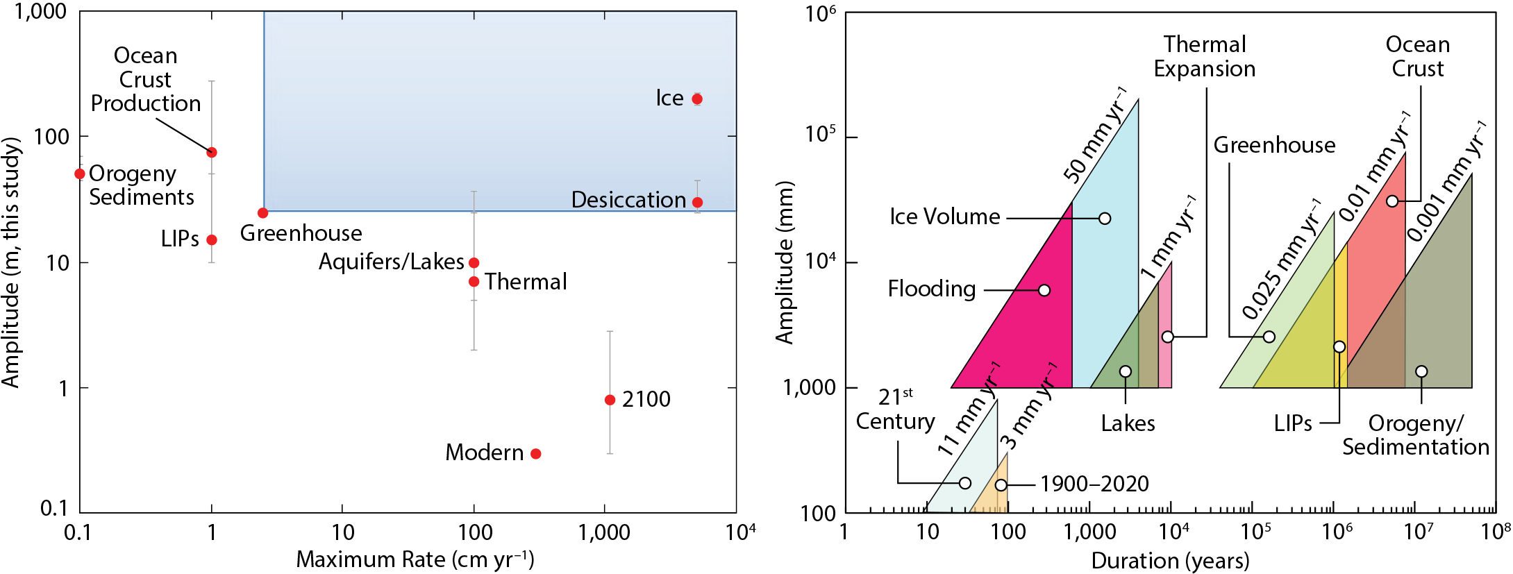
Figure 1. Processes affecting sea level change. (left) Log-log plot of maximum amplitudes (in meters with error) versus maximum rates. The blue box encompasses rates that can only be explained by ice volume changes or basin desiccation. (right) Log-log plot of amplitudes versus durations for each process where the length of each hypotenuse gives the maximum rate of change. LIPs = Large Igneous Provinces. > High res figure

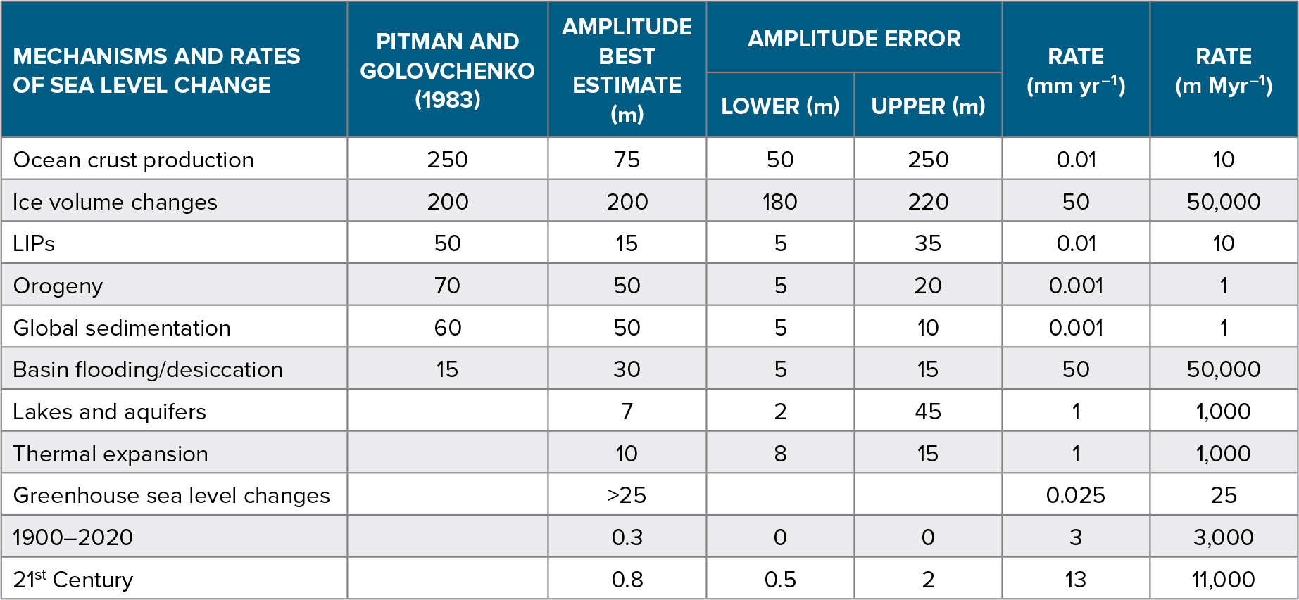
Table 1. Amplitudes and rates of sea level change updated from Pitman and Golovchenko (1983) with best estimates from this study. LIPs = Large Igneous Provinces; the 50 m LIP estimate does not include isostatic loading. > High res table

 

Sea level change is not uniform around the world. Relative sea level (RSL) is the difference in height between the sea surface and the solid Earth at a particular place. GMSL change is the global mean of relative sea level change and is the volume of the ocean divided by the ocean surface area (Gregory et al., 2019). In geological literature, GMSL change is sometimes called “eustatic change,” which is defined with respect to some fixed datum level such as the center of the Earth and is more properly termed global mean geocentric sea level change (Gregory et al., 2019). We eschew the terms “eustasy” and “eustatic change” because such datum levels are lacking or equivocal in the geologic record. RSL change at a particular place is controlled both by GMSL change and by regional and local land motion. RSL includes the effects of thermal subsidence, sediment loading, flexure, mantle dynamic topography, and glacial isostatic adjustment (GIA), as well as changes in the height of the geoid driven by the changing distribution of ice and ocean mass and by GIA. In addition, there are short-term (1–1,000-year scale) ocean dynamic sea level changes (e.g., El Niño and Gulf Stream variations that regionally cause tens of centimeters of transient sea level changes). GMSL variations are caused primarily (Figure 1) by changes in ocean temperature (tens of centimeters on annual to centennial timescales, with up to 10 m over the past 48 million years due to cooling), changes in land ice volume (meter scale operating on decadal to centennial scales and up to 200 m on astronomical timescales of ~20 thousand years [kyr] to 2,400 kyr), and changes in the volumes of ocean basins (100+ m scale primarily on >1 million year timescales; see summary in Miller et al., 2005a).

The yet-to-be formally defined Anthropocene epoch (Zalasiewicz, 2008) can be partly characterized by human-induced modifications of Earth’s climate state due to changes in atmospheric CO₂ concentrations from 280 ppm in ~1850 to 414 ppm in 2020 CE, with current trends projected to lead to 600–900 ppm in this century in the absence of strong global climate policy (Riahi et al., 2017; Meinshausen et al., 2020). Other potential markers for the base of the Anthropocene can be as young as the atomic-testing tritium spike that culminated in 1963, though here we use the CO₂ record to place the base at 1850 CE (Figure 3). The Anthropocene will constitute a climate and sea level state fundamentally different from glacial periods (e.g., 27–20 ka) or the Holocene interglacial (11.3 ka to 1850 CE). Ancient climates range from cold, glacial periods (e.g., Last Glacial Maximum [LGM]) with CO₂ at 180 ppm to warm, ice-free states, the most recent of which are the Early Eocene Climatic Optimum (EECO; 56–48 Ma) and possibly the Miocene Climatic Optimum (17–13.8 Ma), with CO₂ two to three times higher than 1850 CE. Miller et al. (2020) recognize three pre-Anthropocene climate states: Hothouse (very warm, largely ice-free conditions; Late Cretaceous and Early Eocene), cool Greenhouse (Early to Middle Eocene) with small ice sheets (<25 m sea level equivalent), and Icehouse conditions with continental-​scale ice sheets at one or both poles (Figure 2). Today, the Greenland Ice Sheet (GIS) contains 7.4 m of sea level equivalent; the West Antarctic Ice Sheet (WAIS) contains 5.6 m of sea level equivalent, including the Antarctic Peninsula; the East Antarctic Ice Sheet (EAIS) contains 52 m of sea level equivalent; and mountain glaciers and ice caps contain <1 m of sea level equivalent (Morlighem et al., 2019). Within the Icehouse of the Oligocene to Holocene (Figure 2), climates varied on glacial and interglacial timescales, with continental ice sheets waxing and waning in East Antarctica during the Oligocene to Middle Miocene (ca. 34–13.9 Ma), a permanent EAIS developing in the Middle Miocene (ca. 13.8 Ma), and large Northern Hemisphere ice sheets developing in the Quaternary (last 2.55 million years). Changes in ice volume dominate the rise and fall of sea level during Icehouse, cool Greenhouse, and perhaps even Hothouse worlds (Miller et al., 2020).

 

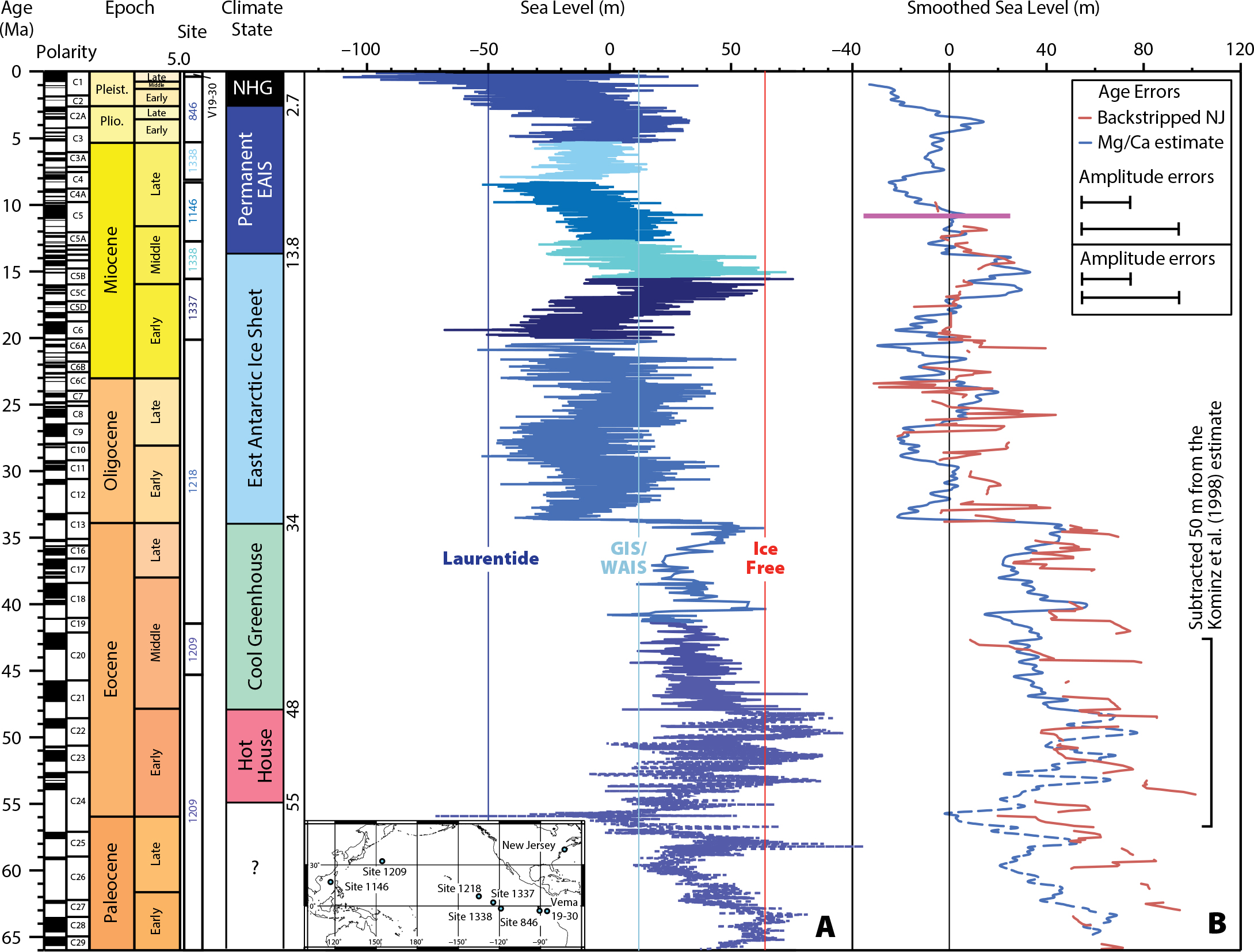
Figure 2. Cenozoic (last 66 million years) sea level, modified after Miller et al. (2020). Timescale is GTS2012 (Gradstein et al., 2012). Sites used in construction of curves are color-coded. Climate states as discussed in text. Inset map shows locations of sites used. (A) Sea level obtained using benthic (Cibicidoides) foraminiferal δ18Obenthic splice and δ18Oseawater using temperatures from Mg/Ca records. The ice-free line (magenta) is drawn 66 m above present, the Greenland Ice Sheet-West Antarctic Ice Sheet (GIS-WAIS; light blue) is drawn at 12 m above present, and the Laurentide Ice Sheet (dark blue) is drawn at –50 m. Each site has a contrasting shade of blue, with the site number indicated in the left column in the corresponding color. The δ18Obenthic splice is based on data from Pacific cores obtained at sites 1209 (Leg 198), 1218 (Leg 199), 1337 (Legs 320/321), 1338 (ODP Legs 320/321), 1145 (Leg 184), 846 (Leg 138) by the Ocean Drilling Program (ODP) and the Integrated Ocean Drilling Program (IODP) and piston core V19-30 (Shackleton et al., 1983); full citations for core collection are available in Miller et al., 2020. The sea level record older than 48 million years is dashed because of uncertainties in the Mg/Ca record (Cramer et al., 2011). Long-term Mg/Caseawater estimates were compiled by Cramer et al. (2011) and a correction for carbonate ion effects was made for the Eocene-Oligocene transition by Miller et al. (2020). Mg/Caseawater estimates are partly the source of uncertainties older than 48 Ma, though the Mg/Ca record older than 48 Ma from Site 1209 is suspect due to high variability (Cramer et al., 2011). (B) Comparison of smoothed sea level estimates from δ18O and Mg/Ca (blue; obtained by interpolating to 20 kyr intervals and using a 49-point Gaussian convolution filter, removing periods shorter than 490 kyr) with backstripped (progressive accounting for the effects of compaction, loading, and thermal subsidence; Miller et al., 2005a; John et al., 2004) onshore New Jersey estimates (red; Kominz et al., 2016). The magenta bar is the range of backstripped sea level change on the Marion Plateau, East Australian margin (John et al., 2004). The New Jersey estimates for the Early to Middle Eocene were shifted by –50 m to compensate for long-term (2–10 million years) effects that are likely due to changes in mantle dynamic topography. > High res figure

 

Measuring Sea Level Changes

Sea level change is determined by measuring time (age) and height of water with respect to datum levels. We refer sea level to the modern mean sea level (MSL) datum level (https://tidesandcurrents.​noaa.gov/datum_options.html). Instrumental measurements of RSL are based on data from tide gauges with extensive global coverage after World War II and sparse coverage dating back to the eighteenth century, and from satellites with global coverage since 1993. GMSL is statistically inferred from these records (e.g., Dangendorf et al., 2017). For reconstruction of ancient sea level, proxies (shorelines, fossils, sediment facies) are calibrated to time and MSL, with ages determined from radiometric data (mostly radiocarbon over the past 40 kyr, with coral U/Th ages back several 100 kyr), from fossils (biostratigraphy), or from other techniques (magnetostratigraphy, chemostratigraphy, and astrochronology). For the Late Pleistocene to present (last 129 kyr), dating of corals or marshes formed near sea level provides the most accurate means or reconstructing sea level. Measurements of foraminifera δ¹⁸O records reflect ice volume and temperature changes that can be calibrated to sea level by independent temperature estimates back through the Middle Eocene (e.g., Miller et al., 2020). Flooding (transgressions) and exposure (regressions) of the continents reflect GMSL and tectonic processes, as does the record of sequences (unconformity bounded units; Vail et al., 1977). Continental flooding and sequence stratigraphy provide the longest (billion year) records, though they also record processes of sediment supply, compaction, loading, thermal and flexural subsidence, mantle dynamic topography, and active tectonics.

Various generations of sea level curves produced by Exxon Production Research Company (Vail et al., 1977; Haq et al., 1987) have become entrenched as the Phanerozoic standard. These “cycle” charts provide an excellent record of the timing of sea level falls but are greatly exaggerated in their sea level amplitudes because they were scaled to sea levels derived from seafloor spreading reconstructions and did not account for processes of compaction, loading, and thermal and flexural subsidence. Even the relative amplitudes are suspect, and thus these curves provide little to no constraints on sea level mechanisms (e.g., Miller et al., 2005a).

Drilling by the International Ocean Discovery Program (IODP) and its predecessors has provided material for independently estimating sea level using sequence stratigraphy and backstripping (progressively accounting for the effects of compaction, loading, and thermal subsidence; John et al., 2004; Miller et al., 2005a), and for combining deep-sea benthic foraminiferal δ¹⁸O and Mg/Ca records, with the latter providing an independent paleothermometer (Lear et al., 2000; Cramer et al., 2011; Miller et al., 2020). Convergence of these two methods (Figure 2B) allows identification of GMSL changes and inferences about their mechanisms (Miller et al., 2020). In addition, coral drilling in Barbados (Figure 3A; Fairbanks, 1989) and Tahiti by IODP Expedition 310 (Deschamps et al., 2012) provides constraints on the rates of sea level rise during the last deglaciation. Finally, studies of Holocene marshes have produced pristine chronologies and estimates of the rates of GMSL rise during the Holocene (Figure 3B), including the CE, that can then be linked to instrument records (tide gauge and satellites). Here, we provide a geological perspective on past, present, and future sea level change using published backstripped (Miller et al., 2020), δ¹⁸O-Mg/Ca (Miller et al., 2020), coral (Peltier and Fairbanks, 2006; Deschamps et al., 2012), marsh (e.g., Kemp et al., 2009, 2018; Kopp et al., 2016; Horton et al., 2018), and instrumental (Dangendorf et al., 2017) sea level records.

 

History of GMSL Changes

High-latitude temperatures were remarkably warm in the Late Cretaceous (e.g., Huber et al., 2018) and Early Eocene (e.g., with Arctic surface temperatures >23°C; Sluijs et al., 2006), and there is consensus that Earth was substantially ice-free at these times, with CO₂ concentrations in excess of 1,000 ppm (summary in Foster et al., 2017). However, sea level records indicate large (>25 m) and rapid changes in the Late Cretaceous to the Eocene that can only be explained by ice growth and decay (e.g., Miller et al., 2005a,b, 2020; Ray et al., 2019; Davies et al., 2020). The solution to this enigma is that there were small (15–25 m sea level equivalent or 25%–40% of modern volume), ephemeral ice sheets during the Late Cretaceous to Eocene in the interior of Antarctica (Miller et al. 2005a; Huber et al., 2018; Ray et al., 2019; Davies et al., 2020). Remarkable new data show marine-terminating glaciers existed at the Sabrina Coast, adjacent to the Aurora Basin, Antarctica, by the Early to Middle Eocene (Gulick et al., 2017), and modeling studies show that significant ice sheets (15+ m equivalent) can exist in regions of high Antarctic topography (Deconto and Pollard, 2003) even while subtropical conditions persist along the coast (Pross et al., 2012). We posit that sea level variations on the order of 15±10 m occurred as significant ice sheets grew and decayed, even in intervals such as the Early Eocene and Late Cretaceous.

The cool Greenhouse conditions of the Middle to Late Eocene illustrate ice volume control on sea level in what was commonly thought to be an ice-free period. Despite warm bottom water temperatures (8°–12°C), our δ¹⁸O-Mg/Ca-based estimates show (Figure 2) large (15–30 m) sea level falls at ca. 49, 47.8, 46.9, and 44.5 Ma; smaller falls (~10–20 m) at 43.6, 42.9, and 40.8 Ma; and a major rise of ~40 m to near ice-free conditions at the Middle Eocene Climatic Optimum (40.1 Ma; Bohaty and Zachos, 2003), followed by a ~20 m drop (39.5 Ma). During the Late Eocene, sea level fell 40 m, only to rise in near ice-free conditions again at ca. 35 Ma. The new Middle to Late Eocene sea level record (Figure 2; Miller et al., 2020) indicates dynamic growth and collapse of moderately large ice sheets (0%–75% of modern EAIS), controlled by the 1,200 kyr tilt cycle (Miller et al., 2020). Atmospheric CO₂ proxies show decreasing values accompanied this change in state (Foster et al., 2017) from Hothouse with ephemeral, small ice sheets to cool Greenhouse conditions with moderate-​​sized ice sheets.

A continental-scale EAIS developed in the Icehouse Early Oligocene associated with Zone Oi1 (ca. 34 Ma; Oi1, Oi2, Mi1 to Mi6 are million-year-scale δ¹⁸O maxima; Miller et al., 1991), with million year sea level falls of 40–60 m and peak glaciations in the Early Oligocene (Oi1, ca. 34 Ma), middle Oligocene (Mi2, ca. 30 Ma), and spanning the Oligocene/Miocene boundary (Mi1, ca. 22 Ma; Miller et al., 2020). Sea level lowstands were generally lower than present from 34–17 Ma, explaining the poor representation of strata of this age in continental margin sections. During this time, ice growth and decay was paced by the 1,200 kyr tilt cycle (Boulila et al., 2011; Miller et al., 2020), though ice volume was affected by the orbital cycles of precession (19/23 kyr), short tilt (41 kyr), and eccentricity (95/125, 405, and 2,400 kyr).

The cool, glacial climates of the Oligocene to Early Miocene were punctuated by the Miocene Climatic Optimum (17.0–13.8 Ma), the last time Earth was potentially ice-free (Miller et al., 2020). The Miocene Climatic Optimum is associated with relatively high CO₂ (~500 ppm), high carbon burial (the Monterey event; Vincent and Berger, 1985), and high global δ¹³C values (though these lag the warming). The Miocene Climatic Optimum may be considered an incipient ocean anoxic event, possibly attributed to outgassing of the Columbia River basalts (Kasbohm and Schone, 2018; Sosdian et al., 2020).

A permanent EAIS developed in the Middle Miocene Climate Transition as signaled by Antarctic climates (Lewis et al., 2008) and three major million year-scale δ¹⁸O_benthic increases, coolings, and attendant sea level falls (Miller et al., 2020): Mi3a (14.8 Ma; ~30 m fall, ~0.7°C cooling), Mi3 (13.8 Ma; ~50 m fall, ~1.2°C cooling), and Mi4 (12.8 Ma; 20–30 m sea level fall, ~1.0°C cooling). GMSL rose after each event but to a lower mean state, stabilizing less than 12 m above present. From 12.8 until ca. 4.5 Ma, the amplitudes of sea level change were muted and ice sheets were mainly paced by the 41 kyr tilt cycle. The large EAIS of the Middle to Late Miocene was less sensitive to precessional and eccentricity forcing. The cause of the Middle Miocene Climate Transition was likely a decrease in atmospheric CO₂ (Greenop et al., 2014), perhaps linked to cessation of Columbia River basalt volcanism and weathering (Sosdian et al., 2020).

The Pliocene recorded the last major warm period (4.5–3 Ma) when (1) global mean surface temperatures were 2°–3°C warmer than 1850 CE (e.g., Dowsett, 2007), (2) CO₂ was similar to 2020 (e.g., Bartoli et al., 2011), and (3) sea levels stood ~22±10 m above present (Miller et al., 2012). Maximum sea level is constrained by δ¹⁸O_benthic values at ca. 3 Ma to <20 m (Miller et al., 2019), though sea level may have peaked higher earlier in the Pliocene (32±5; Hearty et al., 2020). The ~20–30 m estimates are significant because they imply absence of the GIS, the WAIS, and vulnerable portions of the EAIS (Miller et al., 2012). Considering the errors, no melting of the EAIS may be required (Rovere et al., 2014; Raymo et al., 2018). However, sea level estimates generally fall into the range of 15–20 m at 3 Ma and 20–35 m at ca. 3.5–4.5 Ma (Miller et al., 2012, 2019, 2020; Hearty et al., 2020), consistent with melting of the EAIS in the Wilkes and Aurora Basins suggested by models (DeConto and Pollard, 2002) and sediment tracer data (e.g., Bertram et al., 2018; see Gasson and Keisling, 2020). This warmer Early Pliocene world was more sensitive to precessional and eccentricity forcing than the cooler Late Miocene, though the 41 kyr tilt cycle still dominated sea level changes.

Small (Greenland-sized) Northern Hemisphere ice sheets existed at least intermittently beginning in the Middle Eocene (St. John, 2008), but the Quaternary (last 2.55 million years) began with development of continental-scale Northern Hemisphere ice sheets signaled by the large Marine Isotope Stage (MIS) 100 δ¹⁸O increase (>1‰; ~2.5 Ma), sea level fall (~60 m), and appearance of ice rafted sediments in the northern North Atlantic. (MISs are defined as periods of higher [even stages, colder and large ice sheets] and lower [odd stages, warmer, smaller ice sheet] δ¹⁸O values in deep sea carbonates.) Ice sheets gradually increased in size from ca. 2.8–2.55 Ma, with progressive increase in glacial-interglacial δ¹⁸O amplitudes. The cause of the beginning of the large Northern Hemisphere ice ages has been variously attributed to closing gateways (e.g., Panamanian seaway, Norwegian-Greenland sill), mountain building, ocean circulation, and CO₂ drawdown (e.g., discussion in Raymo, 1994), though dropping of CO₂ below a critical threshold of 300 ppm is implicated (Willeit et al., 2015; Miller et al., 2020). Sea level was paced by the 41 kyr tilt cycle with amplitudes <100 m.

Sea level amplitudes increased and began to be paced by short eccentricity (quasi 100 kyr), precession, and tilt forcing during the Bruhnes (780 ka) following the Mid-Pleistocene Transition. Precession (19, 23 kyr) and tilt (41 kyr) directly forced sea level lowerings of 10–60 m, but larger sea level rises yielding the distinct sawtooth 100 kyr terminations of the last 780 kyr are likely due to amplification by CO₂ (Shackleton et al., 2000). The cause of the shift to dominant quasi-100 kyr periods and large, rapid (>100 m) sea level rises during the Mid-Pleistocene Transition is unknown, though decreasing atmospheric CO₂ from ~320 to 250 ppm may have reached a threshold, resulting in the return of a 100 kyr beat that had previously been important in the early history of the EAIS (Miller et al., 2020).

Sea level reached its highest points of the last 780 kyr in MIS 11 (9±3 m, ~405 kyr) and MIS 5 (7.5±1.5 m above present, ca 125 kyr), with global mean temperatures about 1°C warmer than 1850 (Dutton et al., 2015). Sea level reached its lowest point of the last 200 million years during the LGM (Peltier and Fairbanks, 2006; Lambeck et al., 2014). The Barbados sea level record of –120±5 m (Fairbanks, 1989) corrected for GIA indicates the LGM occurred from ~27 ka to 20 ka, with GMSL of 122–127 m below present (Peltier and Fairbanks, 2006). An inversion-​based analysis using over 1,000 sea level observations from corals proposed an LGM timing of 21 ka and GMSL of 134 m, though the database is sparsely populated between 30 ka and 20 ka (Lambeck et al., 2014). Following the LGM, sea level rose with two large Meltwater Pulses, MWP1A (14.7–14.3 ka, rate >47 mm yr^–1) and MWP1B (11.7-11.5 ka, >40 mm yr^–1; Fairbanks, 1989; Stanford et al., 2006; Deschamps et al., 2012; Liu et al., 2016; Abdul et al., 2016).

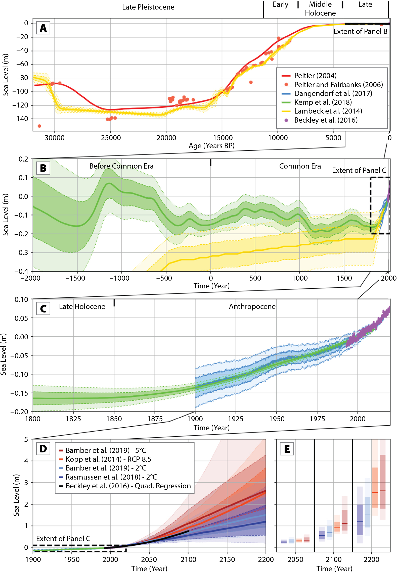
Figure 3. Data sets and statistical analyses of variations in sea level from 30,000 calendar years before 1950 (ka), including the Last Glacial Maximum, 27–20 ka to 2200 CE. Gray correlation lines show the relative temporal relationships between panels. Note that the range varies from over 150 m (panel A) to 60 cm (panel B), 30 cm (panel C), and over 5 m (panels D, E). (A) Time series of global mean sea level (GMSL) estimates from 30,000 calendar years to 1950 (= 0 age). Coral data are from Barbados, corrected for glacial isostatic adjustment (red points; Peltier and Fairbanks, 2006), and the global whole Earth ICE-5G (VM2) model (red line, Peltier, 2004). The GIA-corrected model of Lambeck et al. (2014; yellow line) is shown for comparison. Thick dashed lines/darker shading and thin dashed lines/lighter shading indicate the 1 sigma and 2 sigma errors, respectively, on the statistical estimates of sea level. (B) Time series of GMSL from 2000 BCE to 2020 CE showing statistical analyses of Kemp et al. (2018). Thick dashed lines/darker shading and thin dashed lines/lighter shading indicate the 1 sigma and 2 sigma errors, respectively, on the statistical estimates of sea level. The yellow line is the GIA-corrected model of Lambeck et al. (2014). Blue lines are drawn based on statistical analysis of satellite and tide gauge records by Dangendorf et al. (2019). Purple points indicate satellite data for 1993–2020. (C) Time series of GMSL from 1800 to 2020 based on a statistical analysis of satellite and tide gauge records by Dangendorf et al. (2019; blue line). Purple dots record satellite data for 1993–2020 (Beckley et al., 2016). The green line shows processed combined tide and satellite data. The thick dashed blue line/darker shading and thin dashed blue line/lighter shading indicate the 1 sigma and 2 sigma errors, respectively, on the statistical estimates of sea level.  (D) Time series of GMSL from 1900 to 2200, including process-model sea level projections under 2°C (Rasmussen et al., 2018; Bamber et al. 2019) and 5°C representative concentration pathway (RCP) 8.5 warming scenarios (Kopp et al., 2014, updated for consistency with Oppenheimer et al., 2019; Bamber et al., 2019). The black line is a quadratic regression model fit to the Beckley et al. (2016) satellite data. Extrapolation of the acceleration indicates over 0.7 m of sea level rise by 2100 and a ~12.5 mm yr–1 rate of rise in 2100. Thick dashed lines/darker shading and thin dashed lines/lighter shading represent the 17th to 83rd and 5th to 95th percentiles for each of the sea level projections, respectively. (E) The median 17th to 83rd, and 5th to 95th percentile sea level projections for 2050, 2100, and 2200 from the process-model projection time series displayed in panel D. > High res figure

 

The Holocene (11.3 ka to the beginning of the Anthropocene in 1850 CE) was an epoch of relative stability for global mean temperature and progressive slowing and stabilizing of GMSL. During the Early Holocene (11.3–8.2 ka), GMSL rise slowed to ~8 mm yr^–1 and progressively slowed to 2 mm yr^–1 in the Middle Holocene (8.2–4.2 ka) and less than 1 mm yr^–1 by 5 ka (Figure 3A; Lambeck et al., 2014). Statistical analysis of a global database of regional sea level records (Figure 3B) shows very little change in Late Holocene GMSL (4.2 ka to the beginning of the Anthropocene), aside from hundred-year scale oscillations of ± 0.1 m (Kopp et al., 2016; Kemp et al., 2018). This corroborates the analysis of CE GMSL by Kopp et al. (2016), which exhibited multi-centennial variability of ±0.1 m, but no rising trend. The modern rise is not a remnant of deglaciation but rather due to anthropogenic warming.

The modern period of GMSL rise began in the late nineteenth century, and the rate of rise over the twentieth century was the fastest in at least 3,000 years (Kopp et al. 2016; Kemp et al., 2018). The acceleration of sea level rise continued in the late twentieth and early twenty-first centuries. Statistical analysis of satellite and tide gauge records by Dangendorf et al. (2019) shows a 1.6±0.4 mm yr^–1 rate of sea level rise between 1900 and 2015, with the current acceleration beginning in the late 1960s. The rate of sea level rise increased from 2.1±0.1 mm yr^–1 to 3.4±0.3 mm yr^–1 from 1993 to 2015 (Dangendorf et al., 2017). Using nearly 30 years of satellite data (Nerem et al., 2010; Beckley et al., 2016), a simple regression model (Figure 3C) captures the late twentieth to twenty-first century acceleration of sea level rise. GMSL today is driven primarily by ocean warming (~40%) and the melting of ice sheets (~30%) and mountain glaciers (~20%) (Church et al., 2013; WCRP Global Sea Level Budget Group, 2018).

Though future sea level rise remains a subject of conjecture dependent on future emissions pathways, certain limits can be placed on sea level rise during the twenty-first century and beyond. Simple extrapolation of the acceleration seen in the satellite data (Nerem et al., 2010; Beckley, 2016) predicts over 0.7 m of GMSL rise by 2100 (Figure 3D, thick black line) and a ~12.5 mm yr^–1 rate of rise in 2100. However, whereas the next couple of decades of GMSL rise are independent of emissions pathways, human choices about emissions become an increasingly important driver in the second half of this century and beyond. In a world that eliminates its net carbon dioxide emissions and stabilizes global- mean warming at 2°C above preindustrial temperatures, GMSL is likely (with at least a 66% probability) to be between 0.4 m and 1.0 m by the end of the century (Figure 3D,E; Rasmussen et al., 2018; Bamber et al., 2019). By contrast, in a world of unchecked emissions growth that leads to global-mean warming around 5°C by the end of the century, the currently limited understanding of ice sheet stability on century timescales yields a much broader range of projections. The relatively conservative projections laid out in chapter four of the special report of the Intergovernmental Panel on Climate Change on The Ocean and Cryosphere in a Changing Climate indicate a likely rise of 0.6–1.1 m over this century (Oppenheimer et al., 2019), while a structured expert judgment study (Bamber et al., 2019) indicates a broader range of 0.8–1.7 m.

The future beyond 2100 CE is even less certain. Both process modeling (Clark et al., 2016) and ancient sea level analogs discussed here reflecting slow feedback mechanisms suggest that 2°C of warming will lock in ~10 m of GMSL rise over the coming millennia. Under higher emissions scenarios, twenty-first century GMSL rise greater than 2 m cannot be excluded (e.g., Bamber et al., 2019), and equilibrium rise over the next few millennia may be tens of meters. Emissions to date have committed humanity to a world of sea level rise not seen for 3 million years, and our coastal systems, natural and built, need to adapt, roll back, and continue to acclimate to inexorable rise.

 

Acknowledgments

This work was supported by National Science Foundation grants OCE16-57013 (Miller) and the IODP/Texas A&M Research Foundation. We thank the Office of Advanced Research Computing (OARC) at Rutgers University for providing access to the Amarel cluster and associated research computing resources, IODP for samples, and the IODP community for producing the stable isotope, trace metal, and backstripped data used here. We thank Craig Fulthorpe and Oceanography Associate/Guest Editor Peggy Delaney for reviews.

Miller, K.G., W.J. Schmelz, J.V. Browning, R.E. Kopp, G.S. Mountain, and J.D. Wright. 2020. Ancient sea level as key to the future. Oceanography 33(2):32–41, https://doi.org/10.5670/oceanog.2020.224.

Abdul, N.A., R.A. Mortlock, J.W. Wright, and R.G. Fairbanks. 2016. Younger Dryas sea level and meltwater pulse 1B recorded in Barbados reef crest coral Acropora palmata. Paleoceanography 31:330–344, https://doi.org/​10.1002/2015PA002847.
1. Bamber, J.L., M. Oppenheimer, R.E. Kopp, W.P. Aspinall, and R.M. Cook. 2019. Ice sheet contributions to future sea-level rise from structured expert judgment. Proceedings of the National Academy of Sciences of the United States of America 116:11,195–11,200, https://doi.org/10.1073/pnas.1817205116.
2. Bartoli, G., B. Hönisch, and R.E. Zeebe. 2011. Atmospheric CO₂ decline during the Pliocene intensification of Northern Hemisphere glaciations. Paleoceanography 26(4), https://doi.org/​10.1029/​2010PA002055.
3. Beckley, B., N.P. Zelensky, S.A. Holmes, F.G. Lemoine, R.D. Ray, G.T. Mitchum, S. Desai, and S.T. Brown. 2016. Global mean sea level trend from integrated multi-mission ocean altimeters TOPEX/Poseidon Jason-1 and OSTM/Jason-2 Version 4.2. Ver. 4.2. PO.DAAC, CA, USA. Data set accessed on July 12, 2020 at https://doi.org/10.5067/GMSLM-TJ142.
4. Bertram, R.A., D.J. Wilson, T. van de Flierdt, R.M. McKay, M.O. Patterson, F.J. Jimenez-Espejo, C. Escutia, G.C. Duke, B.I. Taylor-Silva, and C.R. Riesselman. 2018. Pliocene deglacial event timelines and the biogeochemical response offshore Wilkes Subglacial Basin, East Antarctica. Earth and Planetary Science Letters 494:109–116, https://doi.org/10.1016/j.epsl.2018.04.054.
5. Bohaty, S.M., and J.C. Zachos, 2003. Significant Southern Ocean warming event in the late Middle Eocene. Geology 31:1,017–1,020, https://doi.org/​10.1130/G19800.1.
6. Boulila, S., B. Galbrun, K.G. Miller, S.F. Pekar, J.V. Browning, J. Laskar, and J.D. Wright. 2011. On the origin of Cenozoic and Mesozoic “third-order” eustatic sequences. Earth-Science Reviews 109:94–112, https://doi.org/10.1016/​j.earscirev.2011.09.003.
7. Church, J.A., P.U. Clark, A. Cazenave, J.M. Gregory, S. Jevrejeva, A. Levermann, M.A. Merrifield, G.A. Milne, R.S. Nerem, P.D. Nunn, and others. 2013. Sea level change. Pp. 1,137–1,216 in Climate Change 2013: The Physical Science Basis. Contribution of Working Group I to the Fifth Assessment Report of the Intergovernmental Panel on Climate Change. T.F. Stocker, D. Qin, G.-K. Plattner, M. Tignor, S.K. Allen, J. Boschung, A. Nauels, Y. Xia, V. Bex and P.M. Midgley, eds, Cambridge University Press, Cambridge, UK, and New York, NY, USA.
8. Clark, P.U., J.D. Shakun, S.A. Marcott, A.C. Mix, M. Eby, S. Kulp, A. Levermann, G.A. Milne, P.L. Pfister, B.D. Santer, and others. 2016. Consequences of twenty-first-century policy for multi-millennial climate and sea-level change. Nature Climate Change 6:360–369, https://doi.org/10.1038/nclimate2923.
9. Cramer, B.S., K.G. Miller, P.J. Barrett, and J.D. Wright. 2011. Late Cretaceous-Neogene trends in deep ocean temperature and continental ice volume: Reconciling records of benthic foraminiferal geochemistry (δ¹⁸O and Mg/Ca) with sea level history. Journal of Geophysical Research 116(C12), https://doi.org/10.1029/2011JC007255.
10. Dangendorf, S., M. Marco, G. Wöppelmann, C.P. Conrad, T. Frederikse, and R. Riva. 2017. Reassessment of 20^th century global mean sea level rise. Proceedings of the National Academy of Sciences of the United States of America 114:5,946–5,951, https://doi.org/10.1073/pnas.1616007114.
11. Davies, A., B. Greselle, S. Hunter, G. Baines, C. Robson, A.M. Haywood, D.C. Ray, M.D. Simmons, and F.S.P. van Buchem. 2020. Assessing the impact of aquifer-eustasy on short-term Cretaceous sea-level. Cretaceous Research 112:104445, https://doi.org/​10.1016/​j.cretres.2020.104445.
12. DeConto, R.M., and D. Pollard. 2003. A coupled climate-ice sheet modeling approach to the early Cenozoic history of the Antarctic ice sheet. Palaeogeography, Palaeoclimatology, Palaeoecology 198:39–52, https://doi.org/10.1016/S0031-0182(03)00393-6.
13. Deschamps, P., N. Durand, E. Bard, B. Hamelin, G. Camoin, A.L. Thomas, G.M. Henderson, J. Okuno, and Y. Yokoyama. 2012. Ice-sheet collapse and sea-level rise at the Bølling warming 14,600 years ago. Nature 483:559–564, https://doi.org/​10.1038/nature10902.
14. Dowsett, H.J. 2007. The PRISM Palaeoclimate reconstruction and Pliocene sea-surface temperature. Pp. 459–480 in Deep-Time Perspectives on Climate Change: Marrying the Signal from Computer Models and Biological Proxies. M. Williams, A.M. Haywood, J. Gregory, and D.N. Schmidt, eds, The Micropalaeontological Society, Special Publications, The Geological Society, London, UK.
15. Dutton, A., A.E. Carlson, A.J. Long, G.A. Milne, P.U. Clark, R. DeConto, B.P. Horton, S. Rahmstorf, and M.E. Raymo. 2015. Sea-level rise due to polar ice-sheet mass loss during past warm periods. Science 349(6244):aa4019, https://doi.org/10.1126/science.aaa4019.
16. Fairbanks, R.G. 1989. A 17,000-year glacio-​eustatic sea level record: Influence of glacial melting rates on the Younger Dryas event and deep-ocean circulation. Nature 342:637–642, https://doi.org/​10.1038/342637a0.
17. Foster, G.L., D.L. Royer, and D.J. Lunt. 2017. Future climate forcing potentially without precedent in the last 420 million years. Nature Communications 8:1–8, https://doi.org/10.1038/ncomms14845.
18. Gasson, E.G.W., and B.A. Keisling. 2020. The Antarctic ice sheet: A paleoclimate modeling perspective. Oceanography 33:37–46, https://doi.org/10.5670/oceanog.2020.208.
19. Gradstein, F.M., J.G. Ogg, M.D. Schmitz, and G.M. Ogg. 2012. The Geologic Time Scale 2012. Elsevier, New York, NY, 1,176 pp.
20. Greenop, R., G.L. Foster, P.A. Wilson, and C.H. Lear. 2014. Middle Miocene climate instability associated with high-amplitude CO₂ variability. Paleoceanography 29:845–853, https://doi.org/​10.1002/​2014PA002653.
21. Gregory, J.M., S.M. Griffies, C.W. Hughes, J.A. Lowe, J.A. Church, I. Fukimori, N. Gomez, R.E. Kopp, F. Landerer, G. Le Cozannet, and others. 2019. Concepts and terminology for sea level: Mean, variability and change, both local and global. Surveys in Geophysics 40:1,251–1,289, https://doi.org/​10.1007/s10712-019-09525-z.
22. Gulick, S.P.S., A.E. Shevenell, A. Montelli, R. Fernandez, C. Smith, S. Warny, S.M. Bohaty, C. Sjunneskog, A. Leventer, B. Frederick, and D.D. Blankenship. 2017. Initiation and long-term instability of the East Antarctic ice sheet. Nature 552:225–229, https://doi.org/10.1038/nature25026.
23. Haq, B., J. Hardenbol, and P.R. Vail. 1987. Chronology of fluctuating sea levels since the Triassic (250 million years ago to present). Science 235:1,156–1,167, https://doi.org/10.1126/science.235.4793.1156.
24. Hearty, P.J., A. Rovere, M.R. Sandstrom, M.J. O’Leary, D. Roberts, and M.E. Raymo. 2020. Pliocene-Pleistocene stratigraphy and sea-level estimates, Republic of South Africa with implications for a 400 ppmv CO₂ world. Paleoceanography and Paleoclimatology 35:7e2019PA003835, https://doi.org/​10.1029/2019PA003835.
25. Horton, B.P., R.E. Kopp, A.J. Garner, C.C. Hay, N.S. Khan, K. Roy, and T.A. Shaw. 2018. Mapping sea-level change in time, space, and probability. Annual Review of Environment and Resources 43:481–521, https://doi.org/10.1146/annurev-environ-102017-025826.
26. Huber, B.T., K.G. MacLeod, D.K. Watkins, and M.F. Coffin. 2018. The rise and fall of the Cretaceous hot greenhouse climate. Global and Planetary Change 167:1–23, https://doi.org/10.1016/​j.gloplacha.2018.04.004.
27. John, C.M., G.D. Karner, and M. Mutti. 2004. δ¹⁸O and Marion Plateau backstripping: Combining two approaches to constrain late middle Miocene eustatic amplitude. Geology 32:829–832, https://doi.org/10.1130/G20580.1.
28. Kasbohm, J., and B. Schoene. 2018. Rapid eruption of the Columbia River flood basalt and correlation with the mid-Miocene climate optimum. Science Advances 4(9):eaat8223, https://doi.org/10.1126/sciadv.aat8223.
29. Kemp, A.C., B.P. Horton, S.J. Culver, D.R. Corbett, O. van de Plassche, W.C. Gehrels, B.C. Douglas, and A.C. Parnell. 2009. Timing and magnitude of recent accelerated sea-level rise (North Carolina, United States). Geology 37:1,035–1,038, https://doi.org/​10.1130/​G30352A.1.
30. Kemp, A.C., A.J. Wright, R.J. Edwards, R.L. Barnett, M.J. Brain, R.E. Kopp, N. Cahill, B.P. Horton, D.J. Charman, A.D. Hawkes, and others. 2018. Relative sea-level change in Newfoundland, Canada during the past ~3000 years. Quaternary Science Reviews 201:89–110, https://doi.org/​10.1016/​j.quascirev.2018.10.012.
31. Kominz, M.A., K.G. Miller, J.V. Browning, M.E. Katz, and G.S. Mountain. 2016. Miocene relative sea level on the New Jersey shallow continental shelf and coastal plain derived from one-dimensional backstripping: A case for both eustasy and epeirogeny. Geosphere 12:1,437–1,456, https://doi.org/10.1130/GES01241.1.
32. Kopp, R.E., R.M. Horton, C.M. Little, J.X. Mitrovica, M. Oppenheimer, D.J. Rasmussen, B.H. Strauss, and C. Tebaldi. 2014. Probabilistic 21st and 22nd century sea-level projections at a global network of tide gauge sites. Earth’s Future 2:287–306, https://doi.org/10.1002/2014EF000239.
33. Kopp, R.E., A.C. Kemp, K. Bittermann, B.P. Horton, J.P. Donnelly, W.R. Gehrels, C.C. Hay, J.X. Mitrovica, E.D. Morrow, and S. Rahmstorf. 2016. Temperature-driven global sea-level variability in the common era. Proceedings of the National Academy of Sciences of the United States of America 113:E1434–E1441, https://doi.org/10.1073/pnas.1517056113.
34. Lambeck, K., H. Rouby, A. Purcell, Y. Sun, and M. Sambridge. 2014. Sea level and global ice volumes from the Last Glacial Maximum to the Holocene. Proceedings of the National Academy of Sciences of the United States of America 111:15,296–15,303, https://doi.org/10.1073/pnas.1411762111.
35. Lear, C.H., H. Elderfield, and P.A. Wilson. 2000. Cenozoic deep-sea temperatures and global ice volumes from Mg/Ca in benthic foraminiferal calcite. Science 287:269–272, https://doi.org/10.1126/science.287.5451.269.
36. Lewis, A.R., D.R. Marchant, A.C. Ashworth, L. Hedenäs, S.R. Hemming, J.V. Johnson, M.J. Leng, M.L. Machlus, A.E. Newton, J.I. Raine, and others. 2008. Mid-Miocene cooling and the extinction of tundra in continental Antarctica. Proceedings of the National Academy of Sciences of the United States of America 31:10,676–10,680, https://doi.org/​10.1073/pnas.0802501105.
37. Liu, J., G.A. Milne, R.E. Kopp, P.U. Clark, and I. Shennan. 2016. Sea-Level constraints on the amplitude and source distribution of Meltwater Pulse 1A. Nature Geoscience 9:130–134, https://doi.org/​10.1038/NGEO2616.
38. Meinshausen, M., Z.R.J. Nicholls, J. Lewis, M.J. Gidden, E. Vogel, M. Freund, U. Beyerle, C. Gessner, A. Nauels, N. Bauer, and others. 2020. The shared socio-economic pathway (SSP) greenhouse gas concentrations and their extensions to 2500. Geoscientific Model Development 13(8):3,571–3,605, https://doi.org/​10.5194/​gmd-13-3571-2020.
39. Miller, K.G., J.D. Wright, and R.G. Fairbanks. 1991. Unlocking the ice house: Oligocene-Miocene oxygen isotopes, eustasy, and margin erosion. Journal of Geophysical Research 96:6,829–6,848, https://doi.org/10.1029/90JB02015.
40. Miller, K.G., M.A. Kominz, J.V. Browning, J.D. Wright, G.S. Mountain, M.E. Katz, P.J. Sugarman, B.S. Cramer, N. Christie-Blick, and S.F. Pekar. 2005a. The Phanerozoic record of global sea-level change. Science 310:1,293–1,298, https://doi.org/​10.1126/​science.1116412.
41. Miller, K.G., J.D. Wright, and J.V. Browning. 2005b. Visions of ice sheets in a greenhouse world. Marine Geology 217:215–231, https://doi.org/​10.1016/​j.margeo.2005.02.007.
42. Miller, K.G., J.D. Wright, J.V. Browning, A.A. Kulpecz, M.A. Kominz, T.R. Naish, B.S. Cramer, Y. Rosenthal, R.W. Peltier, and S. Sosdian. 2012. High tide of the warm Pliocene: Implications of global sea level for Antarctic deglaciation. Geology 40:407–410, https://doi.org/10.1130/G32869.1.
43. Miller, K.G., M.E. Raymo, J.V. Browning, Y. Rosenthal, and J.D. Wright. 2019. Peak sea level during the warm Pliocene: Errors, limitations, and constraints. PAGES Magazine 27:4–5, https://doi.org/10.22498/pages.27.1.4.
44. Miller, K.G., J.V. Browning, W.J. Schmelz, R.E. Kopp, G.S. Mountain, and J.D. Wright. 2020. Cenozoic sea-level and cryospheric evolution from deep-sea geochemical and continental margin records. Science Advances 6:eaaz1346, https://doi.org/​10.1126/sciadv.aaz1346.
45. Morlighem, M., E. Rignot, T. Binder, D. Blankenship, R. Drews, G. Eagles, O. Eisen, F. Ferraccioli, R. Forsberg, P. Fretwell, and others. 2019. Deep glacial troughs and stabilizing ridges unveiled beneath the margins of the Antarctic ice sheet. Nature Geoscience 13:132–137, https://doi.org/​10.1038/s41561-019-0510-8.
46. Nerem, R.S., D.P. Chambers, C. Choe, and G.T. Mitchum. 2010. Estimating mean sea level change from the TOPEX and Jason altimeter missions. Marine Geodesy 33:435–436, https://doi.org/​10.1080/​01490419.2010.491031.
47. Oppenheimer, M., B.C. Glavovic, J. Hinkel, R. van de Wal, A.K. Magnan, A. Abd-Elgawad, R. Cai, M. Cifuentes Jara, R.M. DeConto, T. Ghosh, and others. 2019. Sea level rise and implications for low-lying islands, coasts and communities. Chapter 4 in IPCC Special Report on the Ocean and Cryosphere in a Changing Climate. H.-O. Pörtner, D.C. Roberts, V. Masson-Delmotte, P. Zhai, M. Tignor, E. Poloczanska, K. Mintenbeck, A. Alegría, M. Nicolai, A. Okem, and others, eds, Cambridge University Press, Cambridge, UK.
48. Peltier, W.R. 2004. Global glacial isostasy and the surface of the ice-age Earth: The ICE-5G (VM2) model and GRACE. Annual Review of Earth and Planetary Sciences 32:111–149, https://doi.org/10.1146/annurev.earth.32.082503.144359.
49. Peltier, W.R., and R.G. Fairbanks. 2006. Global glacial ice volume and Last Glacial Maximum duration from an extended Barbados sea level record. Quaternary Science Reviews 25:3,322–3,337, https://doi.org/10.1016/j.quascirev.2006.04.010.
50. Pitman, W.C. III, and X. Golovchenko. 1983. The effect of sea-level change on the shelf edge and slope of passive margins. Pp. 41–58 in The Shelfbreak: Critical Interface on Continental Margins. D.J. Stanley and G.T. Moore, eds, Society of Economic Paleontologists and Mineralogists Special Publication 33.
51. Pross, J., L. Contreras, P.K. Bijl, D.R. Greenwood, S.M. Bohaty, S. Schouten, J.A. Bendle, U. Röhl, L. Tauxe, J.I. Raine, and others. 2012. Persistent near-tropical warmth on the Antarctic continent during the early Eocene epoch. Nature 488:73–77, https://doi.org/10.1038/nature11300.
52. Rasmussen, D.J., K. Bittermann, M.K. Buchanan, S. Kulp, B.H. Strauss, R.E Kopp, and M. Oppenheimer. 2018. Extreme sea level implications of 1.5°C, 2.0°C, and 2.5°C temperature stabilization targets in the 21^st and 22^nd centuries. Environmental Research Letters 13:034040, https://doi.org/​10.1088/1748-9326/aaac87.
53. Ray, D.C., F.S.P. Van Buchem, G. Baines, A. Davies, B. Gréselle, M.D. Simmons, and C. Robson. 2019. The magnitude and cause of short-term eustatic Cretaceous sea-level change: A synthesis. Earth-Science Reviews 197:102901, https://doi.org/​10.1016/j.earscirev.2019.102901.
54. Raymo, M. 1994. The initiation of Northern Hemisphere glaciation. Annual Review of Earth and Planetary Sciences 22:353–383, https://doi.org/​10.1146/annurev.ea.22.050194.002033.
55. Raymo, M.E., R. Kozdon, D. Evans, L. Lisiecki, and H.L. Ford. 2018. The accuracy of mid-Pliocene δ¹⁸O-based ice volume and sea level reconstructions. Earth-Science Reviews 177:291–302, https://doi.org/​10.1016/j.earscirev.2017.11.022.
56. Riahi, K., D.P. Van Vuuren, E. Kriegler, J. Edmonds, B.C. O’Neill, S. Fujimori, N. Bauer, K. Calvin, R. Dellink, O. Fricko, and others. 2017. The Shared Socioeconomic Pathways and their energy, land use, and greenhouse gas emissions implications: An overview. Global Environmental Change 42:153–168, https://doi.org/10.1016/​j.gloenvcha.2016.05.009.
57. Rovere, A., M.E. Raymo, J.X. Mitrovica, P.J. Hearty, M.J.O. Leary, and J.D. Inglis. 2014. The mid-​Pliocene sea-level conundrum: Glacial isostasy, eustasy and dynamic topography. Earth and Planetary Sciences Letters 387:27–33, https://doi.org/​10.1016/​j.epsl.2013.10.030.
58. Shackleton, N.J., J. Imbrie, and M.A. Hall. 1983. Oxygen and carbon isotope record of East Pacific core V19-30: Implications for the formation of deep water in the late Pleistocene North Atlantic. Earth and Planetary Science Letters 65:233–244, https://doi.org/​10.1016/0012-821X(83)90162-0.
59. Shackleton, N.J. 2000. The 100,000-year ice-age cycle identified and found to lag temperature, carbon dioxide, and orbital eccentricity. Science 289:1,897–1,901, https://doi.org/10.1126/science.289.5486.1897.
60. Sluijs, A., S. Schouten, M. Pagani, M. Woltering, H. Brinkhuis, J.S. Sinninghe Damsté, G.R. Dickens, M. Huber, G.-J. Reichart, R. Stein, and others. 2006. Subtropical Arctic Ocean temperatures during the Palaeocene/Eocene thermal maximum. Nature 441:610–613, https://doi.org/10.1038/nature04668.
61. Sosdian, S.M., T.L. Babila, R. Greenop, G.L. Foster, and C.H. Lear. 2020. Ocean carbon storage across the middle Miocene: A new interpretation for the Monterey Event. Nature Communications 1:134, https://doi.org/10.1038/s41467-019-13792-0.
62. Stanford, J.D., E.J. Rohling, S.E. Hunter, A.P. Roberts, S.O. Rasmussen, E. Bard, J. McManus, and R.G. Fairbanks. 2006. Timing of meltwater pulse 1a and climate responses to meltwater injections. Paleoceanography and Paleoclimatology 21(4), https://doi.org/10.1029/2006PA001340.
63. St. John, K. 2008. Cenozoic ice-rafting history of the central Arctic Ocean: Terrigenous sands on the Lomonosov Ridge. Paleoceanography and Paleoclimatology 23(1), https://doi.org/​10.1029/​2007PA001483.
64. Vail, P.R., R.M. Mitchum Jr., R.G. Todd, J.M. Widmier, S. Thompson III, J.B. Sangree, J.N. Bubb, and W.G. Hatlelid. 1977. Seismic stratigraphy and global changes of sea level: Part 4. Global cycles of relative changes of sea level. Pp. 49–212 in Seismic Stratigraphy: Applications to Hydrocarbon Exploration. C.E. Payton, ed., American Association of Petroleum Geologists Memoir 26.
65. Vincent, E., and W.H. Berger. 1985. Carbon dioxide and polar cooling in the Miocene: The Monterey Hypothesis. Pp. 455–468 in The Carbon Cycle and Atmospheric CO₂: Natural Variations Archean to Present. E.T. Sundquist, and W.S. Broecker, eds, America Geophysical Union, Geophysical Monograph Series, vol. 32, Washington, DC.
66. WCRP Global Sea Level Budget Group. 2018. Global sea-level budget 1993–present. Earth System Science Data 10(3):1,551–1,590, https://doi.org/​10.5194/essd-10-1551-2018.
67. Willeit, M., A. Ganopolski, R. Calov, A. Robinson, and M. Maslin. 2015. The role of CO₂ decline for the onset of Northern Hemisphere glaciation. Quaternary Science Reviews 119:22–34, https://doi.org/​10.1016/j.quascirev.2015.04.015.
68. Zalasiewicz, J., M. Williams, A. Smith, T.L. Barry, A.L. Coe, P.R. Bown, P. Brenchley, D. Cantrill, A. Gale, P. Gibbard, and others. 2008. Are we now living in the Anthropocene? GSA Today 18:4–8, https://doi.org/10.1130/GSAT01802A.1.

This is an open access article made available under the terms of the Creative Commons Attribution 4.0 International License (https://creativecommons.org/licenses/by/4.0/), which permits use, sharing, adaptation, distribution, and reproduction in any medium or format as long as users cite the materials appropriately, provide a link to the Creative Commons license, and indicate the changes that were made to the original content. Images, animations, videos, or other third-party material used in articles are included in the Creative Commons license unless indicated otherwise in a credit line to the material. If the material is not included in the article’s Creative Commons license, users will need to obtain permission directly from the license holder to reproduce the material.