Introduction
Sea surface salinity (SSS) has long been known to be correlated with evaporation and precipitation patterns. However, ocean processes such as mixing and advection can modulate the local salinity balance. The tropical Pacific provides a striking example of the importance oceanic influences have on sea surface salinity. High precipitation associated with the Intertropical Convergence Zone (ITCZ) extends across the tropical Pacific from the western Pacific warm pool to the coasts of Central and South America. In general, the surface salinity field is locally lower beneath this region of highest rain across the Pacific. However, even though the total amount of surface freshwater flux (evaporation minus precipitation) is not dramatically different between the eastern and western ITCZ regions (Lagerloef et al., 2010), the salinity is much lower beneath the ITCZ in the eastern Pacific (e.g., Alory et al., 2012). In addition to the local surface flux and upper-ocean mixing events, advection is also a factor in the upper-ocean salinity balance in the tropical eastern Pacific (Farrar and Plueddemann, 2019, in this issue). Advection in this region is responsible for a mismatch between the locations of the precipitation maximum and the salinity minimum (Delcroix and Henin, 1991).
Precipitation on the ocean’s surface has a stabilizing effect, but may be limited, depending on the regime in which the rainfall occurred: if the wind energy is great enough, the upper ocean entrains underlying water so that changes in upper-ocean salinity will quickly be mixed downward, and can even result in increased surface salinity as more-saline water is mixed upward (Moum et al., 2014). However, conditions can occur in which pronounced rainfall is associated with low-wind situations. In this case, freshwater lenses can form, often on the same horizontal scale as the rain event itself (Tomczak, 1995; Drushka et al., 2019, in this issue). These freshwater pools can affect turbulence in the upper ocean, due to stabilization and rain mixing (Smyth et al., 1997; Zappa et al., 2009). Thus, two regions with similar rainfall amounts, but differing atmospheric mean conditions, may have differing local salinity responses.
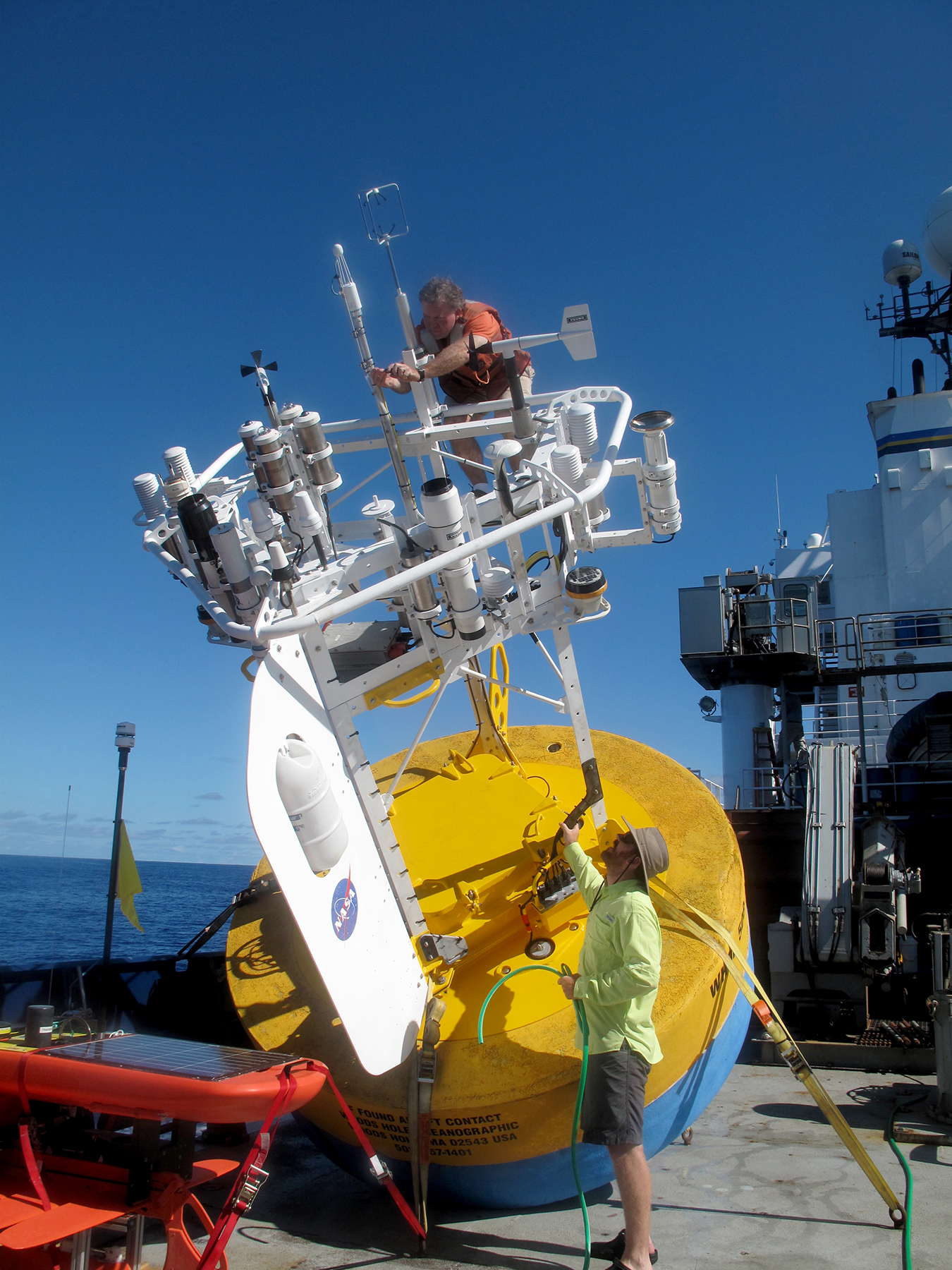
In order to understand variations in the upper-ocean salinity and their relationship to larger-scale atmospheric conditions, a comprehensive set of atmospheric and oceanic data was collected aboard R/V Revelle and from a surface mooring that included a highly instrumented 3 m discus buoy during the Salinity Processes in the Upper-ocean Regional Study (SPURS-2) experiment in the tropical eastern Pacific Ocean. These data include direct estimates of heat, moisture, and momentum fluxes using direct covariance flux systems (DCFSs) on the research vessel and the surface mooring, as well as radiative fluxes and related mean variables measured near the surface and across the coupled boundary layers. These measurements allow us to estimate bulk fluxes, characterize the marine atmospheric boundary layer and the precipitating regimes, and evaluate the effects of precipitation and surface forcing on upper-ocean salinity variability and mixing.
The sections that follow (1) describe the meteorological and near-surface measurements made during the SPURS-2 campaign, (2) explore improvements in estimating evaporation from the ocean surface using direct estimates of moisture flux, (3) investigate the sources and sinks of precipitable water using data from rawinsonde launches, (4) provide examples of how remote sensing can be used to expand these investigations, and (5) study the interplay between solar heating, precipitation, and wind stress and their impacts on ocean mixing using models and SPURS-2 measurements.
Measurement Campaign
The NASA SPURS-2 campaign was conducted in the tropical eastern Pacific Ocean beneath the meandering ITCZ from late August of 2016 to early November of 2017. R/V Revelle deployed the central surface mooring at 10°N, 125°W on August 23, 2016 (Farrar and Plueddemann, 2019, in this issue). After deployment, Revelle conducted a four-week survey to map oceanic temperature, salinity, and velocity fields within a 3° × 3° box about the central mooring. The central mooring was successfully recovered on November 7, 2017. Prior to recovery, Revelle conducted a three-week survey along 125°W between 5°N and 14°N to investigate the meridional variability in the T-S fields beneath the ITCZ (Drushka et al., 2019, in this issue).
“These measurements allow us to estimate bulk fluxes, characterize the marine atmospheric boundary layer and the precipitating regimes, and evaluate the effects of precipitation and surface forcing on upper-ocean salinity variability and mixing.”
Ship-Based Measurements
R/V Revelle was heavily instrumented with meteorological sensors during the deployment and recovery cruises. DCFSs (Edson et al., 1998) were deployed with LI-7500 open-path infrared hygrometers on the forward mast of Revelle during both cruises. The forward mast also supported an optical rain gauge, pressure sensors, and naturally and mechanically aspirated temperature and humidity sensors. Solar and infrared radiometers were deployed at the top of the forward mast during the recovery cruise to place them above the Colorado State University radome (Rutledge et al., 2019, in this issue) and maximize their exposure to downwelling radiation.
Additional instruments were deployed on the forward and aft 02 and 03 decks. These instruments included self-siphoning and manually read rain gauges, pressure sensors, well-exposed solar and infrared radiometers, and a sky camera to document the clouds. A “sea snake” thermistor was deployed off the port side of the ship to measure near bulk sea temperature at approximately 5 cm depth. This instrument provides sea surface temperature (SST, so-called “skin temperature”) after accounting for the cool skin effect (Fairall et al., 1996b). The A-frame over the stern was also instrumented with sonic anemometers and relative humidity and temperature (RH/T) sensors to provide improved measurements while traveling downwind. The fore and aft measurements were calibrated, quality controlled, and used or ignored based on the relative wind direction to minimize the impact of flow distortion and “heat island” effects on the measurements (e.g., measurements were ignored when the relative wind direction was from over the ship for a given set of sensors). A detailed description of the data analysis is given in the SPURS-2 cruise reports and data sources referenced in Bingham et al. (2019, in this issue).
The top three panels in Figure 1 show time series of the temperature, specific humidity, and wind speed for the two cruises where similar conditions were encountered. These variables are used to compute the sensible and latent heat fluxes using the COARE 3.5 algorithm (Edson et al., 2013), discussed in more detail below. The net heat flux was calculated with measured radiative fluxes, estimates of the skin temperature, and calculated latent and sensible heat fluxes as
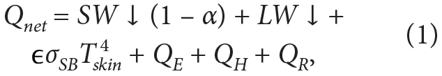
where SW ↓ and LW ↓ are the measured downwelling solar and infrared radiation, α represents the albedo,  approximates the upwelling infrared radiation using the Stefan-Boltzmann law with skin temperature QE and QH the latent heat and sensible heat fluxes, and QR is the sensible heat flux due to rain (Gosnell et al., 1995).
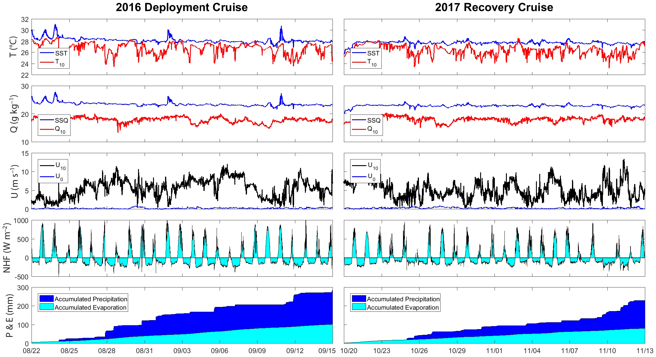
Figure 1. Time series of sea and air temperature, specific humidity, and wind speed (top three panels) measured during the SPURS-2 deployment (left) and recovery (right) cruises. Net heat flux (NHF) computed from the combined radiation measurements, computed sensible and latent heat fluxes, sea surface temperature, and modeled albedo is shown in the fourth panel for each cruise, with a positive value corresponding to heat input to the ocean. Measured precipitation and computed evaporation are shown as accumulations in the bottom panel for each cruise. SST and SSQ are sea surface temperature and specific humidity, respectively; U10, T10, and Q10 are wind speed, temperature, and specific humidity adjusted to 10 m, respectively; and U0 denotes the ocean current adjusted to the surface. Fluxes are as calculated in Equations 1–4. > High res figure
|
The fourth panel displays the net heat flux for the two cruises. Several large positive net heat fluxes occur during periods of light winds, leading to strong diurnal warming (discussed more below). The lower panel provides estimates of accumulated precipitation and evaporation during the cruises. The 2016 cruise experienced wetter conditions with more frequent rain events and stronger evaporation than in 2017, and in general the rain events were associated with stronger winds. Precipitation was approximately three times larger than evaporation during both cruises, with accumulated P−E (precipitation minus evaporation) equal to 182 mm in 2016 and 149 mm in 2017 during the two 24-day periods shown in Figure 1.
Buoy-Based Measurements
The central mooring was also heavily instrumented with meteorological instruments. These included low-power DCFS and redundant Air-Sea Interaction METeorology (ASIMET) sensor packages that measure wind speed and direction, air temperature, pressure and humidity, downwelling solar and infrared radiation, and precipitation. To investigate the salinity budget, the mooring line was instrumented with temperature, salinity, and velocity sensors at multiple depths, as described by Farrar and Plueddemann (2019, in this issue). The redundant sensors and subsurface measurements provided a complete timeline of all variables necessary to estimate the net heat budget from deployment in August 2016 to recovery in November 2017.
The low-power DCFS deployed on the mooring represents the latest version of the autonomous atmospheric turbulent flux package originally developed during the US National Science Foundation (NSF)-sponsored CLIMODE (CLIvar Mode Water Dynamic Experiment) and OOI (Ocean Observatories Initiative) programs. The version developed for SPURS uses a low-cost Gill R3-50 three-axis sonic anemometer and a Lord Microstrain motion sensor interfaced to a microprocessor for system control and higher-order data processing. This version computes motion-corrected fluxes (Edson et al., 1998) in near-real time and telemeters the associated time-mean quantities and turbulent flux estimates to remote users via Iridium.
The key DCFS technological development for SPURS was inclusion of LI-COR infrared gas analyzers to make fast-response humidity measurements, which provide direct measurement of the moisture flux used to estimate latent heat flux and evaporation as defined by Equations 3 and 4 below. An open path LI-7500 was used during SPURS-2 to combat the signal attenuation issues encountered during SPURS-1 using a closed path LI-7200 (e.g., Fratini et al., 2012). The open-path sensor used in SPURS-2 cannot work during rain events, but the rain effectively cleans the optics, and the LI-7500 recovers quickly (i.e., within 20 minutes after the event) to provide direct estimates of moisture flux.
Surface Fluxes and Evaporation
Direct estimates of heat and moisture fluxes can be combined with appropriate state variables to improve parameterization of the transfer coefficients to improve bulk flux estimates. Specifically, the measured (kinematic) moisture,  , and heat,
  , fluxes provide estimates of the sensible and latent heat fluxes as well as surface evaporation from:
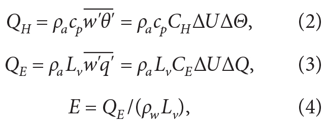
where ρa and ρw are the density of air and water, respectively; cp is the specific heat at constant pressure; Lv is the latent heat of vaporization, w', θ', and q' are turbulent vertical velocity, potential temperature, and specific humidity fluctuations, respectively; CH and CE are the transfer coefficients for heat and moisture known as the Stanton and Dalton numbers, respectively; ΔΘ and ΔQ are the mean sea-air potential temperature and specific humidity differences, respectively; and ΔU is the wind speed relative to the ocean surface (Fairall et al., 1996a). The overbar denotes a time average ranging between 10 minutes and 30 minutes for turbulent fluxes.
The transfer coefficients for latent and sensible heat (i.e., the Dalton and Stanton numbers) provide a means to estimate the heat fluxes using more routinely measured or modeled bulk variables. These bulk estimates of the surface fluxes can then be used for process studies without the need for more difficult-to-measure DC fluxes. The bulk fluxes are also used as lower atmosphere and upper-ocean boundary conditions in most numerical models. In general, these models cannot resolve turbulence near the interface and must parameterize the turbulent fluxes at the air-sea interface.
Improvements to the Dalton and Stanton numbers, however, require direct measurement of the fluxes and the appropriate means given by Equations 2 and 3. The Dalton and Stanton numbers derived from the ship and buoy system during SPURS-1and SPURS-2 are plotted against wind speed in Figure 2. These values have been adjusted to neutral conditions and a height of 10 m using the measured fluxes and the approach provided by Fairall et al. (1996a). The SPURS-1 program was conducted within the salinity maximum of the North Atlantic Ocean where evaporation generally exceeds precipitation (Farrar et al., 2015). The SPURS-1 results are included for comparison with measurements made beneath the ITCZ for SPURS-2 (i.e., two significantly different regimes).
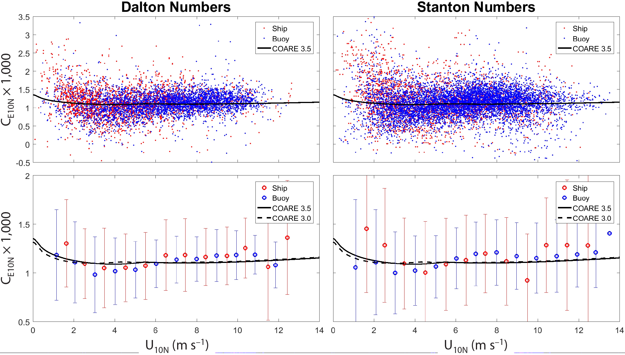
Figure 2. Neutral transfer coefficients adjusted to 10 m for evaporation (CE10N) and heat (CH10N) as a function of the neutral wind speed adjusted to 10 m. The procedure used to adjust measured coefficients to neutral conditions at 10 m is provided by Fairall et al. (1996a, 2003). Symbols shown in red and blue represent ship and buoy data, respectively. The solid and dashed lines represent the parameterization of the transfer coefficients used in the COARE 3.5 and 3.0 bulk algorithms, respectively. The top panels contain all quality-controlled data; the bottom panels show the mean and standard deviation of each coefficient binned into 1 m s–1 wind speed bins. The bins used to average the buoy and ship data have been offset by 0.5 m s–1 to facilitate comparison. > High res figure
|
The coefficients computed using buoy data are shown in blue while the ship data are shown in red. Fast-response humidity measurements on the buoy during SPURS-2 provided the first successful long-duration measurements of moisture flux, and thereby the Dalton number, from a buoy-based system. Previous measurements were confined to research vessel cruises such as those obtained during SPURS-1 and SPURS-2. This lengthy time series roughly doubles the number of direct evaporation measurements ever taken over the ocean, and is a significant achievement of the SPURS-2 program.
The ship and buoy data are in good agreement after correcting for flow distortion as given by Landwehr et al. (2015), except at lower wind speeds where ship-derived transfer coefficients still suffer from flow distortion and heat island effects. The Dalton numbers exhibit less scatter than the Stanton numbers mainly due to larger latent heat fluxes and air-sea specific humidity differences, which provide larger signal to noise ratios. The lower panel shows the COARE 3.0 and 3.5 parameterizations (see Fairall et al., 2003; Edson et al., 2013) of the transfer coefficients where the Stanton and Dalton numbers are assumed identical in these versions; differences between COARE 3.0 and 3.5 are focused mainly on updates to the drag coefficient.
The bin-averaged transfer coefficients from the SPURS buoy and ship-based systems are generally within 10% of the COARE parameterizations in the mean. Consistent with results from other experiments, the current parameterizations appear to slightly overestimate the fluxes at winds below 6 m s–1 and slightly underestimate the fluxes out to approximately 13 m s–1. The SPURS results are expected to reduce the uncertainty in the transfer coefficients at low to moderate winds and will make a significant contribution to the development of COARE 4.0 and more accurate estimates of heat fluxes and surface evaporation.
Atmospheric Soundings
Rawinsondes were launched four times a day to provide atmospheric soundings of temperature, humidity, wind speed, and wind direction during both cruises. Figure 3 displays the average temperature, water vapor mixing ratio, and velocity profiles from the 84 balloon launches conducted during the SPURS-2 deployment cruise. The temperature and humidity profiles are representative of this region of the tropics (e.g., Yuter and Houze, 2000), with a clearly defined tropopause observed at a height of 16 km to 17 km during the deployment cruise (Figure 3). As expected, the humidity profiles show significant variability due to the patchiness in the convection and clouds within the SPURS-2 domain.
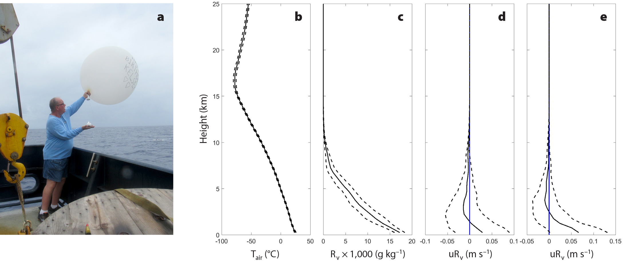
Figure 3. (a) Typical balloon launch from the fantail of R/V Revelle. (b) Average temperature, (c) mixing ratio, and (d) moisture-weighted zonal and (e) meridional wind profiles from the 84 balloon launches. The solid and dashed lines represent the mean and standard deviation of the variables at a given height, respectively. > High res figure
|
The soundings are used to provide estimates of precipitable water in the overlying atmosphere defined as
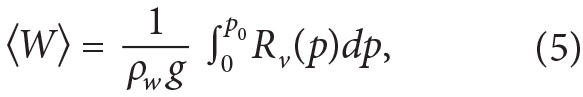
where the brackets are used to denote a vertical integration, g is the acceleration of gravity, ρw is the density of water, and Rv is the mixing ratio for water vapor defined as the ratio of the mass of water vapor to the mass of dry air. As defined by Equation 5, the integration should be performed from the surface pressure, p0, to p = 0. However, as Figure 3 shows, the mixing ratio tends toward zero above 10 km, which is at a pressure level of approximately 290 mb in the tropics. Therefore, this analysis uses all soundings that reach at least 200 mb (~12 km) in our calculations of precipitable water.
The precipitable water and velocity profiles can be combined with our estimates of precipitation and evaporation to investigate the relative importance of evaporation, moisture storage, and moisture flux divergence using the vertically integrated moisture budget (e.g., Dominguez et al., 2006; Brown and Kummerow, 2014):
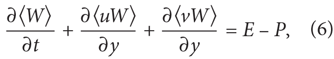
where the terms on the left-hand-side represent the storage term and the vertically integrated horizontal moisture flux divergence (hereafter the moisture flux divergence as in Banacos and Schultz, 2005), with brackets again used to denote vertical integration. The right-hand-side represents the freshwater flux, where E and P are the surface evaporation and precipitation, respectively. The amount of precipitation often exceeds the total amount of precipitable water in the overlying atmosphere. This is a result of moisture flux convergence (i.e., negative divergence) that transports moisture horizontally into a precipitating event from the surrounding area. This is often the case in the equatorial tropical Pacific beneath the ITCZ (Brown and Kummerow, 2014).
The quantities  and
and  represent the vertically integrated moisture-weighted zonal (positive eastward) and meridional (positive northward) moisture flux components. This investigation focuses on the meridional moisture flux divergence under the ITCZ defined as
where the term in brackets is the vertically integrated meridional moisture flux. As with the calculation of precipitable water, this analysis uses all soundings that reach at least 200 mb (~12 km) to compute the moisture flux where the moisture-weighted velocity contribution to the integral becomes small.
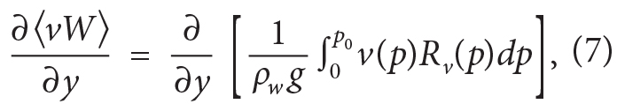
During the first SPURS-2 cruise, the ship conducted a series of meridional transects between 8.5°N and 11.5°N. Roughly eight of these meridional transects were completed every half degree of longitude between 126.5°W and 123.5°W before returning to 125°W to complete one long transect between 5°N and 11°N as shown in Figure 4a. The meridional transects took approximately two days to complete and provided a means to estimate the meridional moisture flux divergence. As Figure 4 shows, this is accomplished by plotting against the meridional distance Y for each transect and applying a linear regression to the data. The slope of the linear regression line provides an estimate of the meridional moisture flux divergence (i.e., = mY + b where m = ∂/∂Y). A negative value of the slope implies moisture flux convergence. These slope-derived estimates of meridional moisture flux divergence show an interesting (and consistent) pattern in Figure 4.
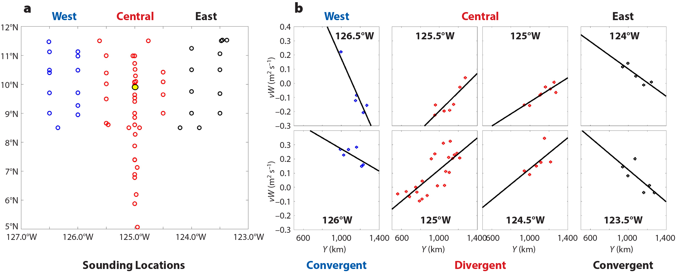
Figure 4. (a) Locations of the soundings (open circles) and the central buoy (yellow dot) during the 2016 cruise. Soundings are identified as west (blue), central (red), or east (black) in relation to the buoy in both the left and right panels. (b) Estimates of the meridional moisture flux as a function of the distance from the equator. The solid lines represent least-square fits to the data where a positive (negative) slope indicates divergence (convergence) according to Equation 7. Each plot corresponds to one of the meridional transects shown in (a) (i.e., two west, four central, and two east). Each plot is identified by the longitude of the transect starting at 126.5°W, moving eastward to 123.5°W before returning to 125°W. The central plot with the largest number of points corresponds to the long transect conducted between 5°N and 11°N along the 125°W transect. The limits of the x-y axes are the same in all subplots for better comparison of the slopes. > High res figure
|
According to this analysis, the buoy was located in a region of moisture flux divergence (positive slope) during this period, typically indicative of patchier (and reduced) rainfall, while to the east and west of the buoy, moisture flux convergence (negative slope) is consistent, typically leading to enhanced rainfall. The divergence over the central region persists even when the ship returns to conduct the last transect along 125°W after approximately a week. The variability in the freshwater flux is dominated by the rate of precipitation in this region, as shown in Figure 1. The mean rate of precipitation varied from 0.69 to 0.46 to 0.45 mm hr–1 for each region moving from west to center to east, respectively, with standard deviations of approximately 4 mm hr–1 using the continuous data shown Figure 1. While not a perfect match, the mean rates are in reasonably good agreement with expected pattern given the variability in rainfall throughout the region.
The overall moisture budget estimated from the sounding data averaged over the four-week cruise provides an estimate of the storage term equal to −0.008 ± 0.278 mm hr–1, the meridional flux divergence term equal to −0.347 ± 2.777 mm hr–1, and the freshwater term equal to −0.372 ± 0.703 mm hr–1, where variability is the standard deviation about the mean. The meridional flux divergence term is derived from the linear fits shown in Figure 4. Likewise, the storage term is derived from linear fits of  against the time taken for each transect. Although the mean of the storage term is near zero, it has the largest variability relative to its mean, consistent with a pattern of discharge and recovery of the moisture in the atmosphere. The variability in the freshwater flux during the eight transects is largely due to variability in precipitation over the region. The variability in the flux divergence during the transects is roughly four times the variability of E−P. Given these large variabilities, the near closure of the moisture budget is quite remarkable.
Satellite Analysis
The zonal pattern seen in the meridional flux divergence is also evident in the moisture budget based solely on satellite observations. Satellite surface salinity observations are available for this time period from NASA’s Soil Moisture Active Passive (SMAP) mission. Satellite precipitation is the Global Precipitation Climatology Project (GPCP; Adler et al., 2018) Version 1.3 Daily Analysis Product, satellite estimates of the surface vector winds are from the Advanced SCATterometer Level-2 (ASCAT-L2; Portabella and Stoffelen, 2009), and satellite estimates of evaporation and mixing ratios (for weighting the surface winds) are from the SeaFlux Climate Data Record V2.0 (Clayson and Brown, 2016). These remotely sensed products were composited to provide daily estimates on a 1° × 1° grid. Figure 5a shows the monthly accumulated freshwater flux total (E−P) and the monthly mean ocean surface salinity during the time period of the first cruise.
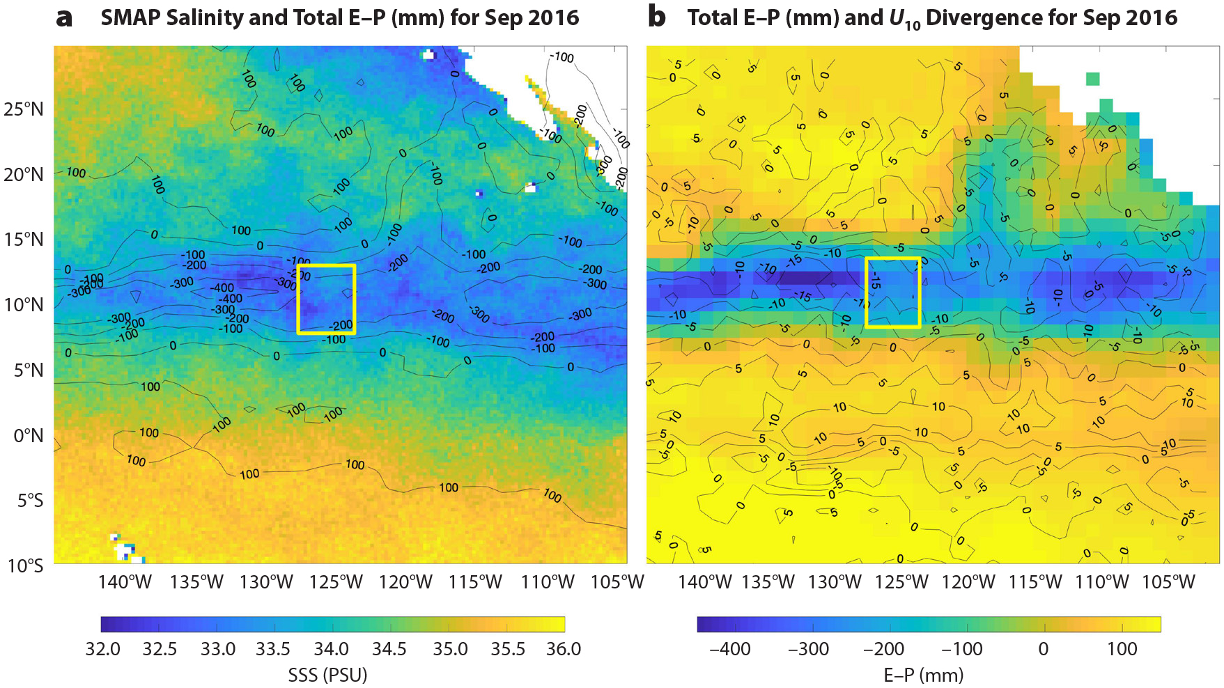
Figure 5. (a) September 2016 average sea surface salinity from the Soil Moisture Active Passive (SMAP) satellite (colors) and estimated evaporation minus precipitation (E–P) from the Global Precipitation Climatology Project (GPCP) and SeaFlux (contours). (b) Estimated E–P from the GPCP and SeaFlux (colors) and divergence estimated from the Advanced SCATterometer (ASCAT). The yellow box indicates the limits of the area covered by the soundings. The rate of evaporation is fairly uniform over this area, such that variability in the accumulated E–P is largely due to precipitation. Less negative E–P is evident in the center of the box due to reduced precipitation, while more negative E–P due to enhanced precipitation is seen in the western and eastern edges of the box. This more-less-more precipitation pattern is consistent with the negative-positive-negative divergence pattern from the soundings shown in Figure 4. > High res figure
|
The close relationship between the surface freshwater flux (E−P) and the ocean salinity in this region is evident from this analysis. The divergence of the moisture weighted surface wind components can be used as a surface proxy for the vertically integrated moisture flux divergence. The close relationship between the freshwater flux and this proxy is also evident in Figure 5b. The regions of moisture flux convergence and divergence as estimated from the ship soundings are also correlated with the observed satellite freshwater flux estimates, with higher precipitation occurring in the western and eastern convergence regions and decreased precipitation over the central divergence region. It should be noted that histograms of the moisture divergence computed from the daily 1° × 1° grid show significant regions of both surface moisture flux divergence and convergence (i.e., negative divergence) beneath the ITCZ. This variability highlights the spatial inhomogeneity of the freshwater flux even within the larger ITCZ precipitation structure.
The measured accumulated E−P during the 24-day deployment cruise is approximately −182 mm (as shown in Figure 1). This value is in good agreement with the monthly averaged satellite-derived estimates of E−P over the SPURS-2 region shown in Figure 5. The monthly averaged satellite estimates of the divergence field using surface winds clearly show moisture convergence beneath the ITCZ. While the monthly average divergence field is too coarse to investigate the negative-positive-negative moisture flux divergence pattern seen in the soundings data (Figure 4), the satellite estimates of E−P show a minimum in the freshwater flux over the SPURS-2 region that is consistent with this divergence pattern (i.e., less rain is expected under moisture flux divergent regions).
Ocean Mixed Layer Observations and Modeling of Precipitating Events
A main focus of the SPURS-2 campaign was to study the effects of precipitation on upper-ocean structure and mixing, and how these localized rain events evolve in the ocean to produce the large-scale salinity structure. Over 800 discrete rain events were captured at the buoy; while most rain events resulted in accumulations of less than 10 mm, 49 of them accumulated more than 20 mm. With this large sample, general patterns relating changes in salinity near the surface with total rainfall and the average wind speed begin to emerge. Figure 6 shows this relationship for near-surface salinity at both 0.95 m and 5.2 m; the clear response near the surface is a function of the rain and the wind, with higher winds leading to reduced surface salinity variability (due to increased downward mixing of the freshwater). At 5 m depth, the salinity response is less than 10% of that observed above, with a less recognizable dependence on wind speed and amount of precipitation.
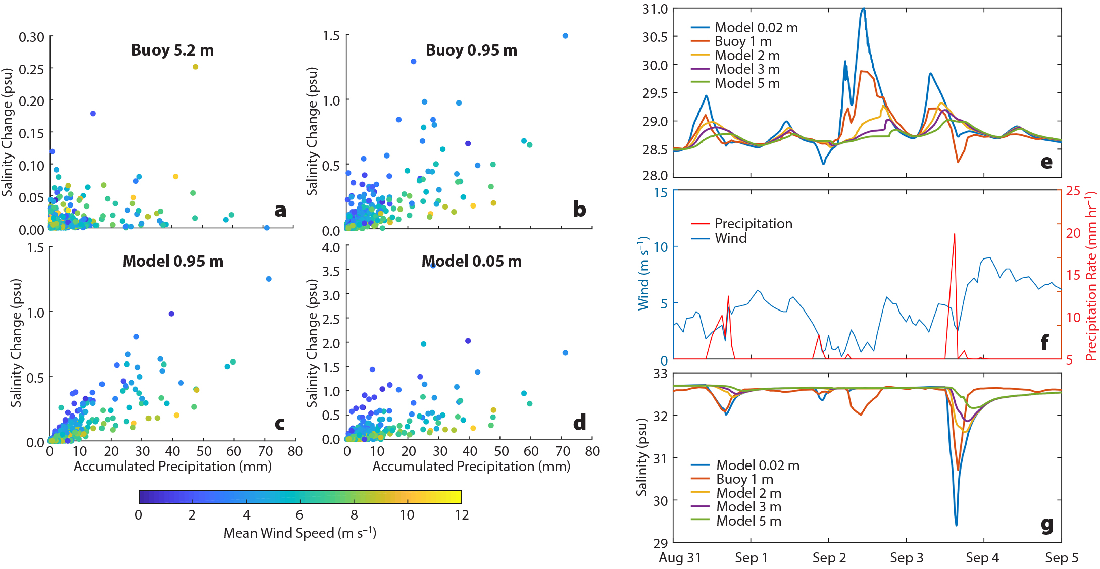
Figure 6. Changes in buoy (a,b) and model (c,d) salinities at various depths as a function of the accumulated precipitation. Colors reflect values of the mean wind speed during the rain event. Model and buoy temperatures (e) and salinities (g) during a five-day period are shown with the associated wind speed and precipitation values (f). > High res figure
|
Figure 6 also shows results from a one-dimensional ocean model initialized by and forced with buoy observations (Kantha and Clayson, 1994, 2004). The model includes wave effects and a parameterization of the rain enhancement of the effective stress. The model is run to 100 m depth for the entire time period when buoy data are available, in four-day simulations that are re-initialized every three days (i.e., the first day of each simulation is not used as the winds are ramped up during this time). The model results at 0.95 m (the same depth as the uppermost buoy level) show a similar dependence on wind speed and rainfall accumulation, with a 0.89 correlation between model and buoy results. At 5 cm from the surface in the model, the freshening is more pronounced for the lightest wind speed cases. Figure 6e–g shows an example of model simulations and buoy observations of several rain events.
The complicated interplay between stabilization of the upper ocean due to diurnal heating and freshwater forcing is also evident. One of the days (September 2) is a low wind, high insolation day, with the expected stratification of temperature in the upper ocean. Although no rain occurs, there is clear advection of fresher water in the buoy signal during this day. Low winds on the following day (September 3) again allow for upper-ocean warming, but the rainfall event beginning near noon brings cold rainwater to the ocean and causes a freshening of over 3 psu very near the surface. The near-surface salinity decrease typically occurs quite rapidly after the onset of precipitation; for instance, the maximum salinity decrease at 0.95 m occurs within the first 10 minutes of the rain event over a third of the time (true for both buoy and model results). Long-lived rain events can have periods of much higher rainfall and so can delay the maximum salinity decrease. This Eulerian view of rainfall impact on the upper ocean is much more abrupt than the Lagrangian view gleaned as the ship steams into and across a freshwater lens during SPURS-2 (e.g., Drushka et al., 2019, in this issue). The modeled maximum salinity decrease occurs later the deeper into the ocean we observe (on average, 20 minutes longer at 5 m than for the near-surface salinity).
The time for the salinity field to recover is, however, a much more complicated process. While the salinity decrease nearest the surface is the largest, and happens much more rapidly, it also tends to take the longest to recover on average. However, there is little coherent relationship between recovery time and accumulated precipitation, average wind, depth, and maximum decrease in salinity. This highlights the difference between rainfall’s immediate local impact on the upper ocean and the larger-scale dynamics and mixing that occurs after formation of a freshwater lens.
Figure 7 shows a sample of rain events occurring at the ship. The same one-dimensional model is used here, with forcing fields taken from the ship observations, and temperature and salinity profiles from the underway CTD casts taken during the cruise. The figure also shows the dissipation from the model (Figure 7d), which provides an estimate of mixing (e.g., Brainerd and Gregg, 1995). The depth to which mixing occurs within the ocean (the mixing layer depth) can be estimated using the dissipation, by examining the depth to which the dissipation decreases to near-background values (in Figure 7, below roughly −7, or  ~ 10–7 m2 s–3) as in Kantha and Clayson (1994) and Sutherland et al. (2014). Again, a strong diurnal warming day is observed on September 1, and mixing is clearly limited to the surface during this stabilization of the upper ocean, with a cascade of the turbulence downward as the ocean begins to cool in the evening (Schudlich and Price, 1992). A few days previously, on August 30, a significant rain event occurs in the morning just as the heating begins. The cool rainwater initially reduces the SST. After the event, the winds stay relatively low and diurnal warming recurs. The following day, August 31, there is again a brief warming time followed by another significant rain event that cools and freshens the surface, followed by gusty winds and intermittent rain events that inhibit diurnal warming. In all of these events, the shallowing of the mixing layer depth is associated with light winds, and, when present, diurnal warming. Although shallow mixing occurs during precipitation, deeper mixing occurs immediately if and when the winds increase following the rain event.
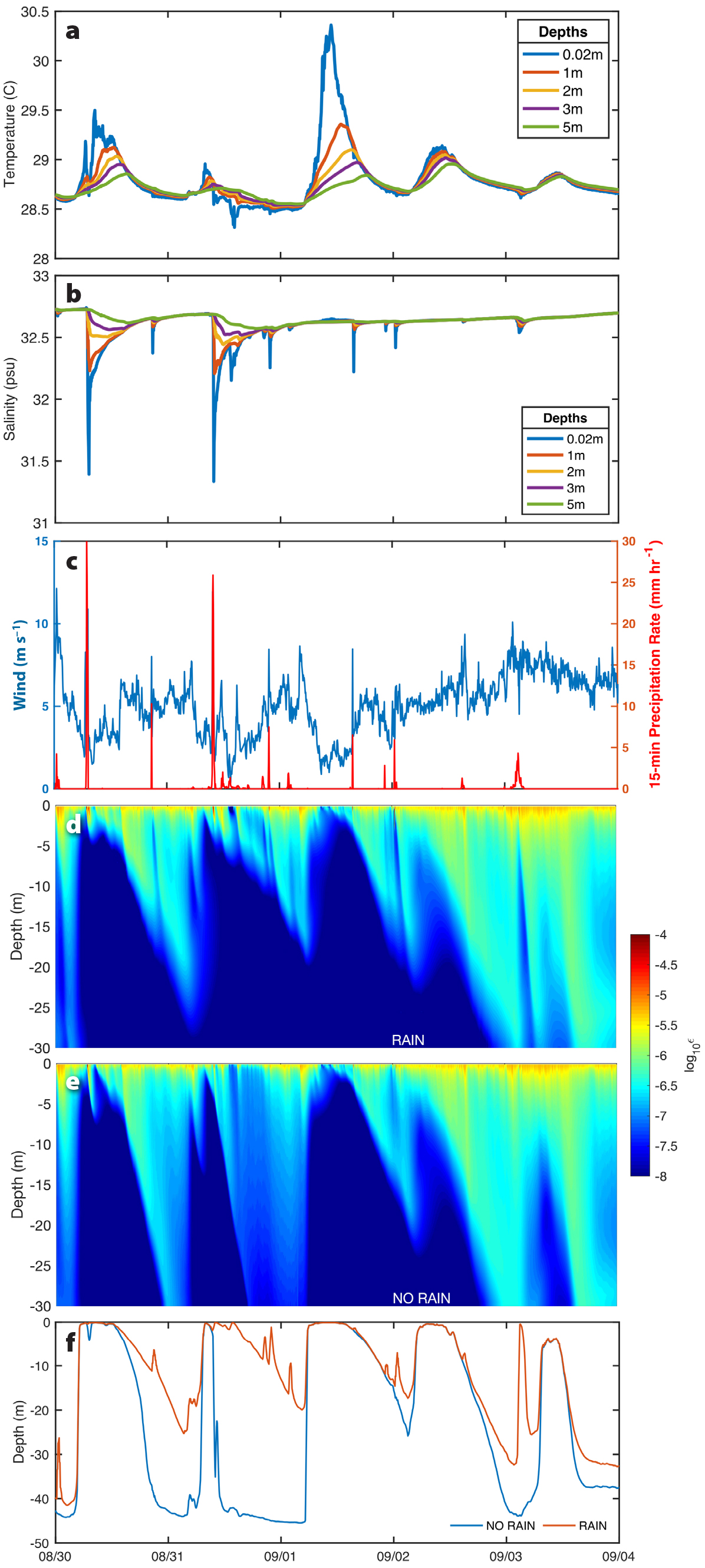
Figure 7. Modeled near-surface temperatures (a) and salinities (b) for several days using data from R/V Revelle measurements (precipitation and wind measurements shown in (c)). Modeled dissipation rates are shown in (d); dissipation rates from a model simulation with no precipitation are shown in (e). Depths of mixing (turbucline depths) are shown in (f); results from the full simulation are shown in red and from the no-rainfall simulation in blue. > High res figure
|
In order to evaluate further the effects of precipitation on upper ocean mixing, an identical model simulation was performed, with one exception: the rainfall was set to zero throughout this time period. Figure 7e shows the resulting mixing. Very little difference in the mixing in the upper 5 m can be seen between the two simulations, although there is some indication of enhanced turbulence in the freshwater region during the rain event. The increase in turbulence within the shallow fresh layer and the decrease below are consistent with the observations of Smyth et al. (1997). However, the freshwater influx does affect the ocean, evidenced by the suppressed mixing below 5 m that occurs in the presence of rainfall and overall freshening of the mixed layer.
Figure 7f shows another way of demonstrating this effect. It displays the difference in the depth at which the surface-induced mixing drops to background levels (defined as the turbucline in Kantha and Clayson, 1994) between the simulation with rainfall (in red) and the simulation without rainfall (in blue). The simulation with rain shows the individual rain events as short duration “spikes” in the turbucline that briefly shallow the mixing depth before being overwhelmed by the wind-driven turbulence. However, by comparing Figure 7d and e, it is clear that the cumulative effect of the rain is felt in the depth of mixing after a shallowing event (occurring through either diurnal warming or rain). This comparison demonstrates that the mixing is shallower with rain than the simulation without rain due to additional stabilization of the upper ocean by the rainfall. Thus, the immediate effect of the rainfall on the very near-surface mixing is typically limited to the rainfall event itself, and is highly dependent on the winds. Nowhere is this more evident than in the precipitation event on September 3 in which the decrease in mixing depth coincides with a sharp decrease in the winds, after which mixing again extends to nearly the depth it was prior to the rainfall event. This complicated interplay of stabilization by warming and rainfall and varying surface momentum input produces a wide variety of mixing scenarios (e.g., Figure 6), and the yearlong SPURS-2 buoy observations will provide fertile ground for further research.
“Measurements of the atmosphere and ocean taken during the SPURS-2 field campaign provide a unique data set for understanding the precipitating region in the tropical eastern Pacific and its relationship with near-surface atmospheric and oceanic variability.”
Concluding Remarks
Measurements of the atmosphere and ocean taken during the SPURS-2 field campaign provide a unique data set for understanding the precipitating region in the tropical eastern Pacific and its relationship with near-surface atmospheric and oceanic variability. Contemporaneous measurements of the atmospheric boundary layer, the ocean boundary layer, and surface fluxes permit evaluation of the effects of rainfall on upper-ocean structure and mixing. The patchy and episodic rainfall observed at the buoy is a result of atmospheric conditions related to moisture flux divergence and storage. Resulting near-surface salinity stratification during the rain events is clear, but the evolution of the salinity stratification is strongly modulated by net heat flux and surface stress (i.e., wind mixing). Overall reduction of mixing at depth due to enhanced stratification is driven by continued input of freshwater to the upper ocean, which is clear from observations and simulations using a turbulence resolving mixed-layer model.
Although SPURS-2 focused on the tropical eastern Pacific, results from the data discussed here are more widely applicable. In particular, the direct measurements of heat and moisture fluxes from the buoy add significantly to our knowledge of air-sea transfer of moisture and heat and will help improve bulk formulas. The good agreement between ship and satellite observations of the atmosphere and the ocean surface provide confidence in the use of observations to investigate how local processes impact the coupled ocean-atmosphere system on larger scales.