Paleoceanography is changing from a qualitative story-telling field to one that is quantitative. This transformation is in part due to the development and adoption of a growing arsenal of statistical tools that evaluate uncertainty. A strength of the field is the illustration of fundamental changes in the Earth/ocean/climate system that are beyond humanity’s recent experience. A weakness lurks in the difficulty of telling time well. Precise and accurate geochronology is essential for establishing rates of change and for quantifying physical or biogeochemical fluxes.

Rates and fluxes are important constraints on the impacts of carbon (and other) feedbacks on a warming climate. We know that additional warming of the planet is already “baked into” our future because paleoceanographers and paleoclimatologists have documented how the relatively long response times of the ocean’s interior, ice sheets, and some carbon reservoirs slow down the various responses to forcings (e.g., carbon emissions)—but may also eventually amplify them or render them irreversible; thus, we know that new Earth system equilibria will only be approached after millennia. For example, over 90% of the excess heat produced by artificially elevated CO₂ is already in the ocean (Durack et al., 2018). If humanity eventually controls its carbon emissions and reduces atmospheric CO₂, it will take a long time for the excess heat to emerge from, and for the excess carbon to be neutralized in, the ocean (Ehlert and Zickfeld, 2018).

 

Fortunately, progress is at hand. Radiometric age models are improving. For example, Marine20, a new calibration of marine radiocarbon data into so-called “calendar” ages, is just out and now extends back ~55,000 years (Heaton et al., 2020). The details remain tricky and model-dependent in the ocean because of the need to account for the changing carbon cycle coupled to changes in circulation patterns and rates in the ocean interior, which conspire with changing ¹⁴C production rates to influence regional reservoir ages. The model that projects Marine20’s surface-water reservoir ages over the past 55,000 years propagates uncertainties in changing ¹⁴C production and carbon cycling, while satisfying constraints of limited data available from the ocean. This is a big improvement over previous syntheses. Nevertheless, the representation of changing deep-ocean circulation is inevitably incomplete. We do not yet know this history because various tracers do not yet converge on a single answer without re-evaluation of processes that control the tracer measurements including δ¹³C and εNd (Du et al., 2020), and this too has implications for radiocarbon reservoir ages.But how fast and how much will our planet change? To answer those questions, we need paleo studies that better constrain transient times and feedbacks so models can be adequately tested under extreme change scenarios and better predict the future with confidence. Fischer et al. (2018) summarized various impacts of past warming on the scale of a few degrees of global warming above preindustrial levels, but avoided specifying rates of change, considering them too uncertain with available chronological constraints.

Marine20 comes with a clear warning that it applies to the warm surface ocean assumed to be near dynamic equilibrium with respect to ocean mixing and air-sea gas exchange. Application to higher latitudes or regions of changing wind-driven upwelling, where these assumptions break down, requires additional considerations, such as assignment of a deviation from the ideal reservoir age, known as Delta-R, which varies regionally. Delta-R may also vary through time, but for lack of constraints, it is often assumed constant through time. Efforts are underway to use a variety of simple models to begin to address this issue empirically (e.g., Walczak et al., in press).

A continuous age model based on radiocarbon or other sources of age datums involves finding a logical pathway between dated levels, with quantified uncertainties. Several Bayesian tools are available to assist in this task, such as Bacon (Blaauw and Christian, 2011), Bchron (Haslett and Parnell, 2008; Parnell, 2020), and Oxcal (Bronk Ramsey, 2009). Quantitative correlation also now provides for assessment of the precision of stratigraphic alignment of “wiggly” proxy signals as an adjunct to independent chronologic information (Lee et al., 2019).

These Bayesian methods, now widely used, are not limited to radiocarbon but can be used with many kinds of data for alignment and as smart interpolation tools with propagation of uncertainties. Their solutions are not all identical, however. Tools like this don’t absolve us of thinking carefully about the systems we are measuring and the assumptions underlying the methods, which may include ideas about sedim‑entation patterns and mechanisms.

Assigning sediment accumulation rates is unfortunately not as simple as taking a first derivative of an age model curve, and may be subject to circular reasoning if sedimentation processes are assumed as part of the age modeling exercise. The sedimentary record’s completeness is thought to be a function of the time span over which it is measured (Sadler and Strauss, 1990); specifically, longer time integrations tend to have lower apparent sediment accumulation rates because of a higher probability of missing sediment. Point-by-point flux normalization notwithstanding (e.g., by ³He or ²³⁰Th; e.g., Costa et al., 2020), a reasonable requirement for minimizing missing-sediment bias is to calculate sediment accumulation rates over fixed and constant time intervals while propagating quantified uncertainties in the age models from the Bayesian age modeling tools. This is relatively straightforward using Monte-Carlo bootstrap methods, but is rarely done.

Calculation of biogeochemical fluxes demands further error propagation of sediment accumulation, bulk densities, and component concentrations. This is accomplished by binning or otherwise assessing proxy data within the boundaries of the time intervals for averaging, and convolving bin uncertainties on dry bulk density with those on property concentrations and sedimentation rates. This too is sufficiently complicated that bootstrap methods are reasonable approaches. The literature is rife with examples of calculated fluxes made with point data applied to interpolated ages between age datums of unequal spacing and without error propagation.

To illustrate how point spacing effects, binning, and changing resolution affect inferred changes in mass accumulation rates and their uncertainties, I calculated carbon burial fluxes (Figure 1) using a published high-resolution data set from a well-characterized core in the Northeast Pacific off Oregon (W98709-13pc, 42.117°N, 125.750°W, 2,712 m depth, with an average spacing between dated levels of 500 years; Lopes et al., 2015). That study showed apparent decoupling between diatom-based primary productivity, export productivity, and organic carbon burial in response to climate change, and it raised questions about how to address issues concerning the effects of biogeochemical fluxes on carbon feedbacks in climate models.
 

Figure 1. Illustration of various model assumptions used in calculating organic carbon mass accumulation rates (MAR: a convolution of sedimentation rate from calibrated dates, dry bulk density, and organic carbon [Corg] contents, using data compiled by Lopes et al., 2015, here recalibrated with the Marine20 calibration curve of Heaton et al., 2020). (a) Age-depth curve with Bayesian age model calculated using Bchron (Parnell, 2020). Organic carbon mass accumulation rates calculated using (b) point-to-point MAR changes based on all Marine20 calendar dates (black) and as a sensitivity test every second date odd (red) and even (blue). (c) Point-to-point MAR changes based on Bchron’s Bayesian age model at the dated levels, otherwise as in (b). (d, e, f) Bootstrap calculations with full uncertainty propagation for Corg MAR in 500-, 1,000-, and 2,000-year bins, respectively. The result in (b) is unstable, and age reversals produce negative MAR, requiring arbitrary decisions about data culling. The result in (c) is better, because the Bayesian model resolves age reversals, but uneven spacing imposes resolution bias. The uniform bins in (d, e, f) allow uncertainty estimation and illustrate the trade-offs between resolution and certainty—coarser time bins give more certain results, but may lose important temporal structure. > High res figure

 

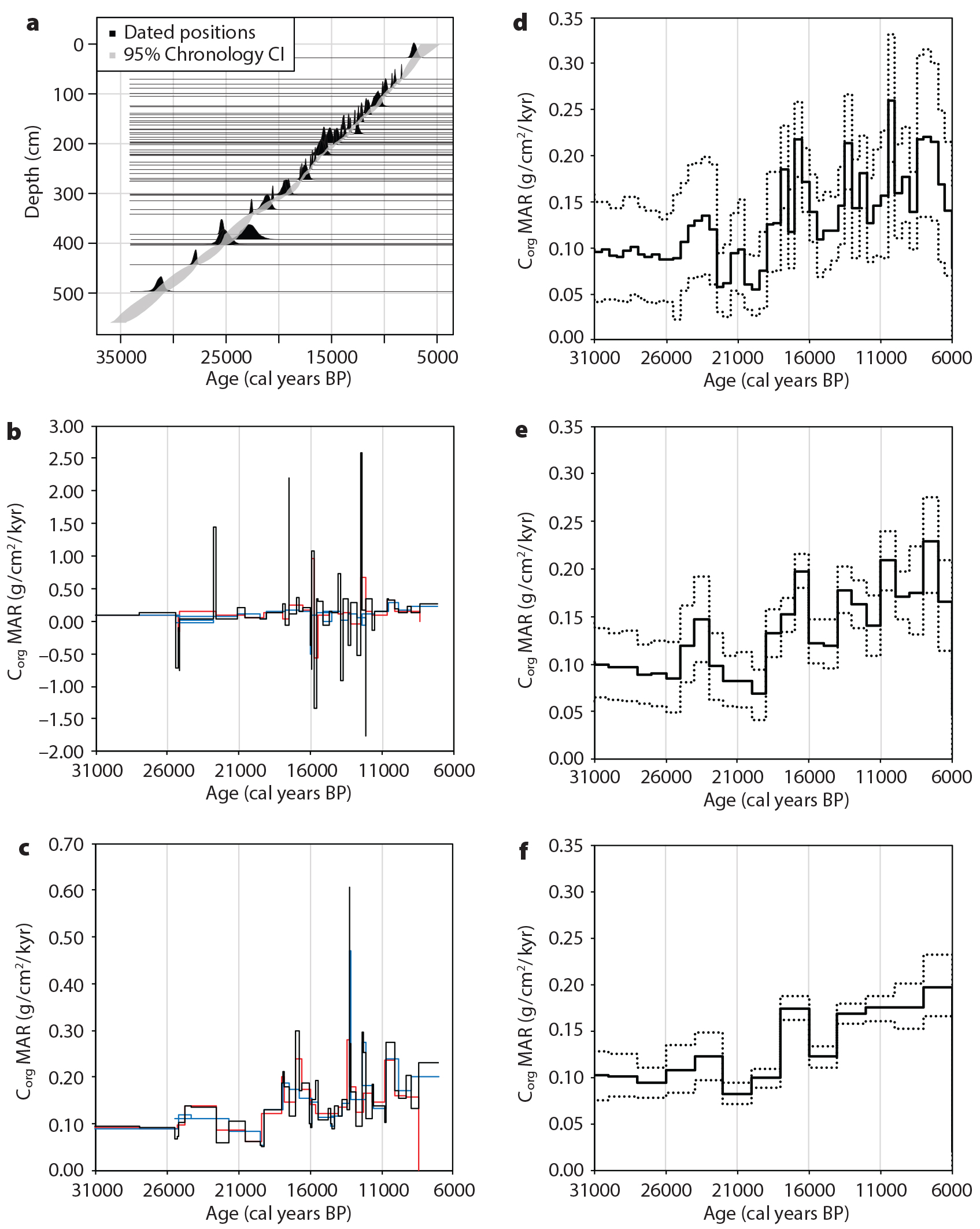
In this case, it appears that variations in carbon burial are not resolved beyond uncertainty in 500-year bins, that some events appear to be resolved in 1,000-year bins, and that most variations are resolved in 2,000-year bins. Armed with this analysis, it is possible to choose at what reasonable temporal resolution and what significance level to evaluate changes in biogeochemical fluxes, or before analysis, we can determine how to design a sampling and analysis program to get the resolution and precision needed to test a hypothesis.

Among paleoceanography’s grand challenges for the coming decade is to refine geochronology, and in so doing to quantify rates of change and material fluxes. To do this well demands understanding of biases in the sedimentary record and rigorous estimation of uncertainties. While a variety of approaches will probably always be needed, widespread adoption of new and emerging Bayesian age modeling tools is essential. Quantitative estimation of uncertainty reveals the need for higher-resolution and higher-precision data sets, which put further demands on our laboratories, and of course on the funding that pays for the analyses. We can expect these approaches to continue to evolve and improve as the relevant literature of theory, tools, and applications expands.

Mix, A.C. 2020. On quantifying stratigraphic, chronologic, and paleo flux uncertainties in paleoceanography. Oceanography 33(2):29–31, https://doi.org/10.5670/oceanog.2020.223.

Blaauw, M., and J.A. Christen. 2011. Flexible paleoclimate age-depth models using an autoregressive gamma process. Bayesian Analysis 6(3):457–474, https://doi.org/10.1214/11-BA618.

Bronk Ramsey, C. 2009. Bayesian analysis of radiocarbon dates. Radiocarbon 51(1):337–360, https://doi.org/10.1017/S0033822200033865.

Costa, K.M., C.T. Hayes, R.F. Anderson, F.J. Pavia, A. Bausch, F. Deng, J.C. Dutay, W. Geibert, C. Heinze, G. Henderson, and others. 2020. ²³⁰Th normalization: New insights on an essential tool for quantifying sedimentary fluxes in the modern and Quaternary ocean. Paleoceanography and Paleoclimatology 35:e2019PA003820, https://doi.org/​10.1029/​2019PA003820.

Du, J., B.A. Haley, and A.C. Mix. 2020. Evolution of the global overturning circulation since the Last Glacial Maximum based on marine authigenic neodymium isotopes. Quaternary Science Reviews 241:106396, https://doi.org/​10.1016/j.quascirev.2020.106396.

Durack, P.J., P.J. Gleckler, S.G. Purkey, G.C. Johnson, J.M. Lyman, and T.P. Boyer. 2018. Ocean warming: From the surface to the deep in observations and models. Oceanography 31(2):41–51, https://doi.org/10.5670/oceanog.2018.227.

Ehlert, D., and K. Zickfeld. 2018. Irreversible ocean thermal expansion under carbon dioxide removal. Earth System Dynamics 9(1):197–210, https://doi.org/​10.5194/esd-9-197-2018.

Fischer, H., K.J. Meissner, A.C. Mix, N.J. Abram, J. Austermann, V. Brovkin, E. Capron, D. Colombaroli, A.-L. Daniau, K.A. Dyez, and others. 2018. Palaeoclimate constraints on the impact of 2°C anthropogenic warming and beyond. Nature Geoscience 11:474–485, https://doi.org/10.1038/s41561-018-0146-0.

Haslett, J., and A. Parnell. 2008. A simple monotone process with application to radiocarbon-dated depth chronologies. Journal of the Royal Statistical Society, Series C 57(4):399–418, https://doi.org/​10.1111/​j.1467-9876.2008.00623.x.

Heaton, T.J., P.R. Köhler, M. Butzin, E. Bard, R.W. Reimer, W.E.N. Austin, C. Bronk Ramsey, P.M. Grootes, K.A. Hughen, B. Kromer, and others. 2020. Marine20: The marine radiocarbon age calibration curve (0–55,000 cal BP). Radiocarbon, https://doi.org/10.1017/RDC.2020.68.

Lee, T., L.E. Lisiecki, D. Rand, G. Gebbie, C.E. Lawrence. 2019. Dual proxy Gaussian Process stack: Integrating δ¹⁸O benthic and radiocarbon proxies for inferring ages on ocean sediment cores. arXiv preprint, https://arxiv.org/pdf/1907.08738.pdf.

Lopes, C., M. Kucera, and A.C. Mix. 2015. Climate change decouples oceanic primary and export productivity and organic carbon burial. Proceedings of the National Academy of Sciences of the United States of America 112(2):332–335, https://doi.org/10.1073/pnas.1410480111.

Parnell, A. 2020. Package ‘Bchron’, https://cran.r-project.org/web/packages/Bchron/Bchron.pdf.

Sadler, P.M., and D.J. Strauss. 1990. Estimation of completeness of stratigraphical sections using empirical data and theoretical models. Journal of the Geological Society 147:471–485, https://doi.org/10.1144/gsjgs.147.3.0471.

Walczak, M.H., A.C. Mix, E.A. Cowan, S. Fallon, L.K. Fifield, J. Alder, J. Du, B. Haley, T. Hobern, J. Padman, and others. In press. Phasing of millennial-​scale climate variability in the Pacific and Atlantic Oceans. Science, https://doi.org/10.1126/science.aba7096.

This is an open access article made available under the terms of the Creative Commons Attribution 4.0 International License (https://creativecommons.org/licenses/by/4.0/), which permits use, sharing, adaptation, distribution, and reproduction in any medium or format as long as users cite the materials appropriately, provide a link to the Creative Commons license, and indicate the changes that were made to the original content. Images, animations, videos, or other third-party material used in articles are included in the Creative Commons license unless indicated otherwise in a credit line to the material. If the material is not included in the article’s Creative Commons license, users will need to obtain permission directly from the license holder to reproduce the material.