Sea surface salinity (SSS) observations from NASA’s satellite missions, Aquarius/SAC-D and Soil Moisture Active Passive (SMAP), are used to describe spatial patterns of the seasonal cycle, as well as intraseasonal and interannual variability, in the eastern tropical Pacific, the location of the second Salinity Processes in the Upper-ocean Regional Study (SPURS-2) field experiment. The results indicate that the distribution of SSS variance is highly inhomogeneous in both space and time. The seasonal signal is largest in the core of the Eastern Pacific Fresh Pool and in the Gulf of Panama. The interannual signal is highest in a relatively narrow zonal band along approximately 5°N, while the intraseasonal signal appears to be a dominant mode of variability in the zonally stretched near-equatorial region. Located right in the middle of a hotspot of high SSS variance, the SPURS-2 site appears to be at the crossroads of many different processes that shape the distribution of SSS in the eastern tropical Pacific and beyond.

 

INTRODUCTION

Sea surface salinity (SSS) is a key variable that reflects changes in the intensity of the global water cycle and plays an important role in ocean dynamics. Knowledge of the spatial and temporal distribution of SSS is essential for climate monitoring (US CLIVAR Office, 2007). Moreover, in order to understand and predict changes in the water cycle and the global climate system, improved understanding of the processes that control distribution of salinity in the ocean is necessary. To study these processes, NASA initiated a field program, Salinity Processes in the Upper-ocean Regional Study (SPURS). The first phase of the program, SPURS-1, took place in the subtropical North Atlantic in 2012–2013, focusing on a “dry,” evaporation-​dominated regime of the subtropical SSS maximum (Lindstrom et al., 2015). The second phase, SPURS-2, was conducted in 2016–2017 in a rainy area in the eastern tropical Pacific, focusing on a “wet,” rainfall-dominated regime of the tropical SSS minimum (SPURS-2 Planning Group, 2015). The two phases were thus designed to cover both source and sink regions of the ocean freshwater cycle. Here, we focus on SPURS-2, which has just been completed in the eastern tropical Pacific, providing a plethora of new, exciting, and very diverse multiplatform data (Bingham et al., 2019, in this issue).

The eastern tropical Pacific is an important region in the global climate system, exhibiting variability over a broad range of spatial and temporal scales. In significant part, this variability is related to El Niño-Southern Oscillation (ENSO) events that affect weather and climate patterns around the world (McPhaden et al., 2006), so it is not surprising that this region has been a subject of intensive study (Fiedler and Talley, 2006; Kessler, 2006). Ocean salinity, however, remains one of the least understood components of ocean and climate variability, in part because of a scarcity of salinity observations in the past (US CLIVAR Office, 2007).

Until recently, our knowledge of SSS distribution and variability, particularly in the tropical ocean, was based on a compilation of sparse and irregularly sampled observations obtained mostly from ships of opportunity (Delcroix and Henin, 1991; Alory et al., 2012). The situation has changed in the last decade with the expansion of the Argo program; yet the Argo array, with its nominal sampling of one profile in a 3° longitude by 3° latitude box every 10 days, remains insufficient to resolve important features and variability, such as fronts, waves, eddies, and intraseasonal variability.

The salinity observing system has been considerably improved through high-resolution observations of SSS from orbiting satellites. Since 2010, satellite instruments have been providing near-global, detailed observations of SSS, resulting in new knowledge about SSS variability and the processes that control it. NASA’s Aquarius satellite was launched in June 2011 and operated for nearly four years (August 2011– May 2015), providing SSS observations with unprecedented spatial and temporal coverage. NASA’s Soil Moisture Active Passive (SMAP) satellite was launched in January 2015 and, though SSS monitoring was not its prime mission objective, has provided quite accurate SSS data over the global ocean, continuing the legacy of Aquarius. These SSS data are complemented by measurements from the European Space Agency’s Soil Moisture and Ocean Salinity (SMOS) satellite launched in November 2009.

The satellite-based observations of SSS provide considerably more spatial detail of SSS variability and its temporal evolution than any in situ component of the global ocean observing system. More importantly, satellite observations provide continuous time series and synoptic views over the global ocean. Based on these capabilities, the aim of this paper is to present a concise description of SSS variability in the eastern tropical Pacific as observed by NASA’s satellites, providing a large-scale context for studies related to in situ measurements from the SPURS-2 field campaign. Our study is based on a Level-4 SSS product that merges Aquarius and SMAP observations into a continuous and consistent multi-satellite SSS data record. From this product, we describe spatial patterns of the mean seasonal cycle, as well as intraseasonal and interannual variations, the latter being dominated by the 2015–2016 El Niño event. The following sections provide details on data and methodology, results, and conclusions.

 

DATA AND METHODOLOGY

To describe SSS variability in the region, we use the multi-satellite SSS data set developed at the University of Hawai‘i in collaboration with Remote Sensing Systems (RSS). The data set merges observations from two NASA satellite missions and covers the period from September 2011 through August 2018. The beginning segment, covering the period from September 2011 to June 2015, utilizes data from the Aquarius satellite and is based on the optimum interpolation analysis (OI SSS; Melnichenko et al., 2016). The analysis is produced on a 0.25° grid and uses a dedicated bias-correction algorithm to correct the satellite retrievals for large-scale biases with respect to in situ data. The time series is continued with the SMAP satellite-based SSS data provided by RSS. To ensure consistency and continuity in the data record, SMAP SSS fields are adjusted using a set of optimally designed spatial filters to correct the data set for large-scale biases (only static [time-mean] biases for each satellite are explicitly corrected) and, at the same time, reduce small-scale noise. During the overlapping period (April–May 2015), the data from the two satellites are averaged to produce a continuous time series. The consistency and accuracy of the new SSS data set has been evaluated against in situ salinity from Argo floats and the Tropical Atmosphere Ocean (TAO) buoy array. A more detailed description of the Aquarius/SMAP SSS data set and the evaluation statistics can be found in Melnichenko et al. (2018). Digital data used in the analysis are available online at http://iprc.soest.hawaii.edu/users/oleg/oisss/ETP/.

Additional observational data have been used to connect the observed SSS variability to the hydrological cycle. These include precipitation data from the Global Precipitation Climatology Project (GPCP; Huffman et al., 2016; https://rda.ucar.edu/​datasets/​ds728.3/), evaporation data from the Objectively Analyzed air-sea Fluxes project (OAFlux; Yu and Weller, 2007; http://oaflux.​whoi.edu), mixed layer depth from the Asia-Pacific Data Research Center (APDRC) Products based on Argo data (http://apdrc.soest.hawaii.edu/projects/argo/), and surface currents from the Ocean Surface Current Analyses Realtime (OSCAR) data set (https://www.esr.org/research/oscar/oscar-surface-currents/).

Time series of SSS at each grid point were divided into interannual, seasonal, and intraseasonal components. Interannual SSS variations were estimated by filtering the weekly time series at each grid point with a 12-month half-width Hanning filter. The seasonal cycle at each grid point was modeled as the sum of the annual and semi-annual harmonics least-squares fitted to the time series (e.g., Bingham et al., 2010):

where S₀ is the mean, t is time measured in days since January 1, 2011, ω₁₂ and ω₆ are the annual and semiannual frequencies (ω₁₂ = 2π/12 months, ω₆ = 2π/6 months), and A₁₂, A₆, φ₁₂, and φ₆ are the amplitudes and phases. The intraseasonal variations were estimated by high-pass filtering the weekly time series of SSS with a six-month half-width Hanning filter.

For each component, we present spatial patterns of the standard deviation (a measure of the magnitude of variability) and the proportion of variance explained by each component, in order to assess to what degree each component contributes to the total signal. The spatial patterns are presented as the corresponding SSS and SSS anomaly maps at seasonal and interannual timescales. Propagation of features is assessed from Hovmöller diagrams, showing SSS anomalies as a function of one spatial dimension (either longitude or latitude) and time.

 

RESULTS

Background

The seven-year mean SSS (Figure 1a) reflects mainly large-scale features described in previous studies (e.g., Fiedler and Talley, 2006). The Eastern Pacific Fresh Pool (EPFP), delineated by the 34 psu isohaline, extends as a low-​salinity tongue from the coast of Central America to the west, reaching 140°W at about 10°N. Salinity in the fresh pool progressively decreases toward the east; the lowest salinities, lower than 33 psu, are found close to the coast in the Gulf of Panama, forming the far eastern Pacific fresh pool. Here, the lowest salinity forms due to summer monsoon rainfall and associated river runoff (Alory et al., 2012). To the west, the fresh pool stretches along the mean position of the Intertropical Convergence Zone (ITCZ), but with a 2°–3° latitude shift to the north from its axis (red dashed line). This satellite-​observed relative distribution of the SSS minimum and the ITCZ is remarkably consistent with that reported by Tchilibou et al. (2015) and inferred from more than 30 years of in situ SSS data. The meridional shift is mainly due to ocean currents, which push low-salinity waters, formed under rainy conditions, northward (Delcroix and Henin, 1991; Yu, 2014).

Figure 1b maps the standard deviation in SSS. The largest values, up to 1 psu, are found close to the coast in the Gulf of Panama. Relatively large values are also found in a zonal band between 6°N at 100°W and 12°N at 130°W. The eastern part of this band corresponds to the mean position of the ITCZ. Further west, the largest values of the standard deviation, up to 0.5 psu, are in the area surrounding the SPURS-2 central site at 10°N, 125°W. This variability, however, consists of multiple temporal and spatial scales, as discussed below.

 

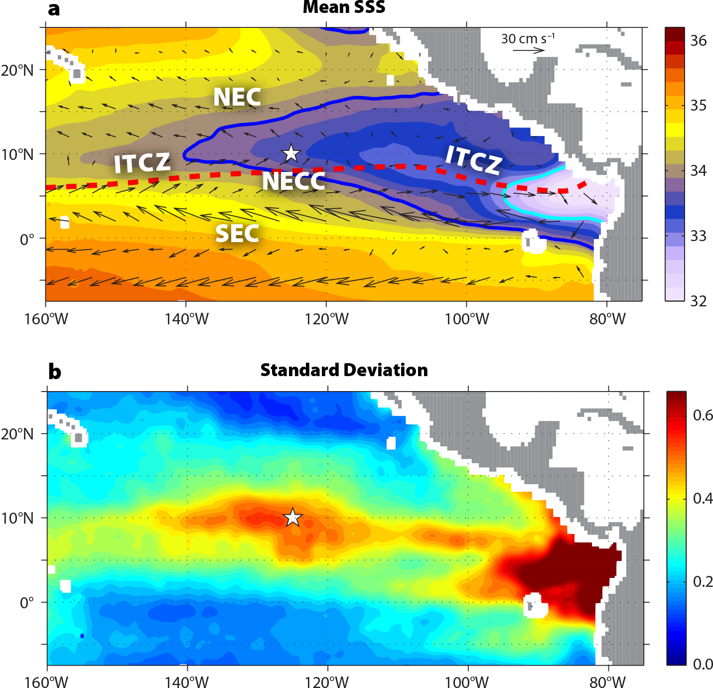
Figure 1. (a) Seven-year mean sea surface salinity (SSS) in the eastern tropical Pacific. Contour interval is 0.2 psu. Enhanced color contours are 34 psu (blue) and 33 psu (cyan). The white star at 10°N, 125°W shows the location of the central mooring during the SPURS-2 field campaign. The red dashed line approximates the mean position of the Intertropical Convergence Zone (ITCZ) defined as the location of the maximum rainfall from the 2011–2017 mean Global Precipitation Climatology Project (GPCP) data. Arrows show seven-year mean currents from the Ocean Surface Current Analyses Realtime (OSCAR) data set. NEC = North Equatorial Current. SEC = South Equatorial Current. NECC = North Equatorial Countercurrent. (b) The standard deviation of SSS computed from weekly time series of Aquarius/Soil Moisture Active Passive (SMAP) SSS for the period September 2011 through August 2018. > High res figure

 

We now decompose the total variability into the three components, as described in the Data and Methodology section, and plot in Figure 2 the distributions of the standard deviation and the fraction of variance for each component to show where each component dominates. We can see that the associated geographical patterns are very different from each other and from that of the total variability (Figure 1b).

 

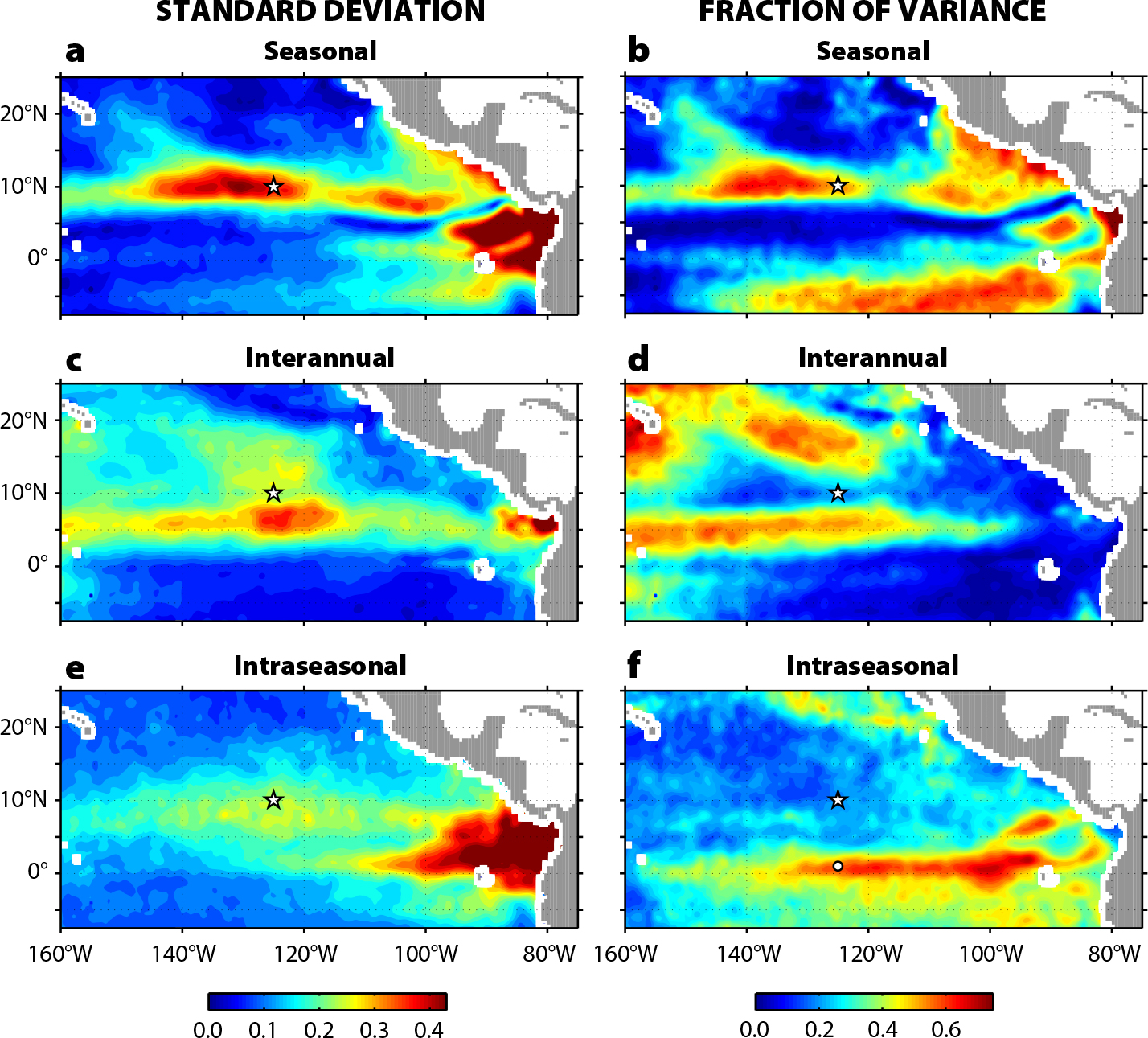
Figure 2. Standard deviation and fraction of total SSS variance contributed by (a–b) seasonal cycle, (c–d) interannual variations, and (e–f) intraseasonal variability. The white star at 125°W, 10°N shows the location of the SPURS-2 central mooring. In the SPURS-2 domain, seasonal variability accounts for about 55% of the total SSS variance. Second in significance is intraseasonal variability, amounting to about 22% of the total variance, and the third is interannual signal, ~18%. The rest, ~5%, can be attributed to the residual seasonal cycle not captured by the fitted annual and semi-annual harmonics. The white circle in (f) marks the location of the SSS time series shown in Figure 6a. > High res figure

The standard deviation of the SSS seasonal cycle (Figure 2a) ranges from near zero to 1 psu. The largest values (>0.5 psu) are found in two areas. A relatively narrow ribbon of high variability can be observed along approximately 8°–12°N between 145°W and 90°W, likely associated with a region of heavy rains under the seasonally varying ITCZ. Another region of significant seasonal variability is in the Gulf of Panama. Here, the amplitude of the annual cycle is the largest, reaching 1 psu. A relatively large seasonal signal of up to 0.4 psu is found near the coast of Central America between approximately 5°N and 15°N. The seasonal signal produced in the rest of the region is quite small, less than 0.2 psu.

To assess to what degree the annual cycle in SSS is representative of the total signal, Figure 2b shows the fraction of variance of the weekly time series explained by the seasonal cycle. There are large regions where the seasonal cycle is a dominant signal despite the small amplitude, such as along ~5°S in the southern part of the domain. Likewise, there are areas where the seasonal cycle accounts for less than 25% of the total SSS variance despite the large amplitude. One such area is in the far eastern fresh pool, where the amplitude of the seasonal cycle is the largest in the region, while the contribution of this seasonal cycle to the total signal can be lower than 50% in some places, pointing to a possible interplay between processes of different timescales.

The second dominant mode of SSS variability in the region is interannual variability, which exceeds 0.3 psu in two locations: most notably along the zonal band centered at ~7°–8°N (Figure 2c), slightly equatorward of the SPURS-2 site, and in the Gulf of Panama, where the amplitude of SSS interannual variations is comparable to or even larger than that of the seasonal cycle. In terms of contribution to the total variance, the zonal band of high interannual variability extends westward along ~5°N, amounting to more than 50% of the total variability west of 120°W. Interannual variations also contribute the majority of the total variance in the region around the Hawaiian Islands and in a tongue of high relative variability to the north of the SPURS-2 domain. The latter is in part because of the relatively weak seasonal and intraseasonal variability throughout this area (Figure 2b,f).

Intraseasonal variability with periods shorter than six months is another example of the differential distribution of the absolute magnitude and the relative contribution to the total signal. While the largest amplitudes, up to 0.5 psu, are observed in the far eastern fresh pool, east of about 110°W (Figure 2e), the intraseasonal variations constitute a dominant mode of variability in a zonally stretched near-equatorial region, between about 4°S and 4°N and 150°W and 90°W (Figure 2f). The SPURS-2 site at 125°W, 10°N shows quite large amplitudes of intraseasonal variations, up to 0.2 psu, yet their contribution to the total variance is low, less than 25%, as the annual signal dominates the time series there (Figure 2a).

 

Spatial Patterns of Seasonal Variability

We begin with the spatial patterns of seasonal variability. The mean SSS in the region ranges from 32 psu in the EPFP to ~36 psu in the subtropics (Figure 1a). The magnitude of seasonal variations is from 0.1 to 1 psu (Figure 2a). These relatively small variations have a dramatic effect on the structure and size of the EPFP (Guimbard et al., 2017). Figure 3 therefore shows both the seasonal SSS fields (multiyear mean SSS plus seasonal anomalies) and seasonal anomalies. The SSS fields allow examination of the evolution of the fresh pool, focusing on its geometry and size, as in Guimbard et al. (2017). The anomaly patterns offer a more nuanced view compared to the simpler patterns of the SSS fields themselves, allowing us to trace propagating features and determine in detail how the spatial patterns of seasonal variability evolve.

 

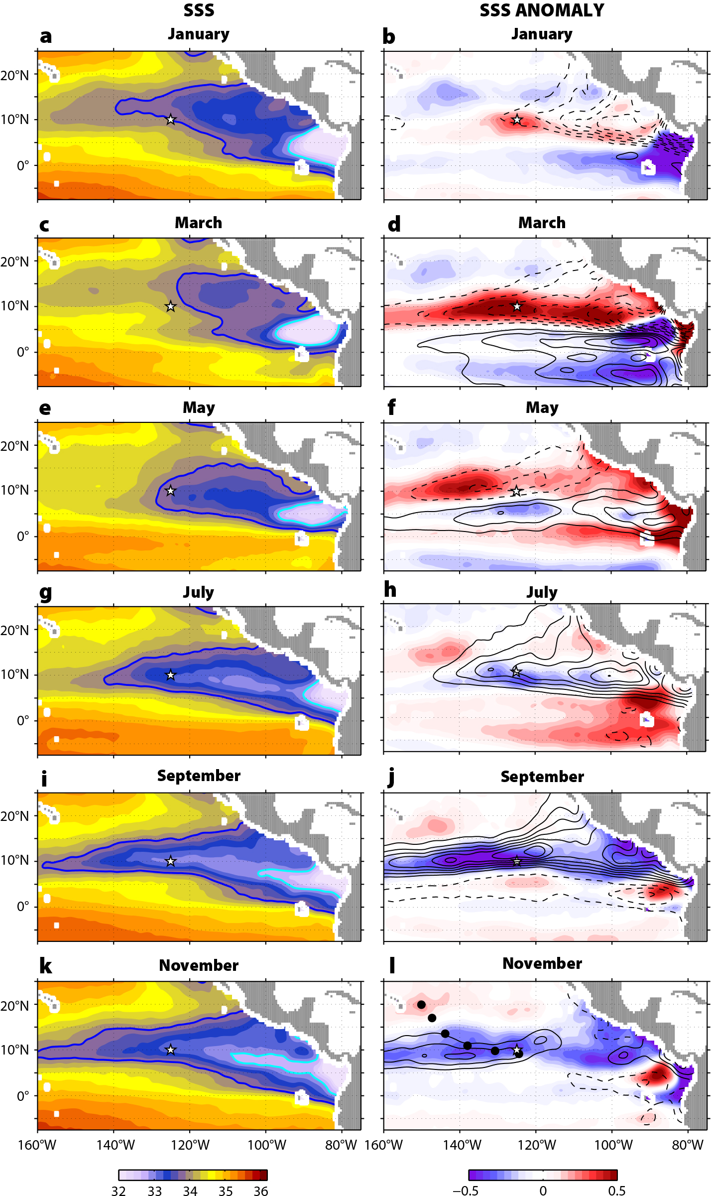
Figure 3. Spatial patterns of seasonal SSS variability in the eastern tropical Pacific: SSS and SSS anomaly for (a,b) January, (c,d) March, (e,f) May, (g,h) July, (i,j) September, and (k,l) November. Contours in the right panels show seasonal anomalies of the freshwater flux term (S0(E – P)/h). Solid contours indicate negative anomalies (precipitation exceeds evaporation), and dashed contours indicate positive anomalies (evaporation exceeds precipitation). Contour interval is 0.05 psu/month; zero contour is omitted. Black dots in panel (l) track the path of the positive SSS anomaly observed at 10°N in January (panel b). > High res figure

 

To explore the seasonal dynamics of the EPFP, Guimbard et al. (2017) computed climatological monthly mean SSS from the five years (2010–2015) of SMOS SSS data. It is therefore useful to compare the results from Aquarius/SMAP over a different period (2011–2017) with those obtained by Guimbard et al. (2017) to see if the results reveal new features. We find that the large-scale patterns are very similar, indicating that the SSS seasonal cycle and the spatial patterns associated with it are robust over the sampling period and from different instruments. The EPFP has the least westward extent, at ~120^oW, and is weakest in March. The freshest region is in the Gulf of Panama at the eastern end of the pool. The pool then gradually strengthens and grows westward along a northwest-southeast oriented band, roughly coinciding with the mean ITCZ east of ~110^oW (Figure 1a, red dashed line), and along ~10°N west of 110°W. While progressing westward, the fresh pool remains narrow, occupying 4°–8° of latitude, which explains why the pattern of dominant seasonality in Figure 2a is so localized in latitude. In this progression, the SPURS-2 site is right in the middle of its path, so the annual cycle is the dominant signal there. The fresh pool reaches its greatest westward extent at ~170°W and is freshest during the September to November period, then begins to erode. The low-salinity waters are pushed northward by the wind-driven ocean currents (Yu, 2014), so we can see the residual fresh water along ~14°N in March (Figure 3c), when a new cycle begins.

The anomaly fields offer quite a different perspective. We begin our description with a zonally elongated positive SSS anomaly observed in January in the vicinity of the SPURS-2 site (Figure 3b). From January to March, the anomaly intensifies considerably and spreads in a zonal band along ~10°N. The anomaly also shifts west-northwestward, presumably being advected by ocean currents (Figure 1a). Tracing this anomaly over the next nine-month period (in Figure 3l, the dots mark the path of the anomaly), we find that by the end of the year it reaches 20°N, thus entering the subtropical gyre. Although considerably weakened by this time, being of the order of 0.1 psu, the anomaly is still significant given the fact that the amplitude of the SSS seasonal cycle in the subtropical gyre barely exceeds 0.1 psu (Gordon et al., 2015). Following the annual cycle, negative anomalies appear south of the SPURS-2 site in May–June (Figure 3f) and then follow the same path of propagation. It is important to remember that the seasonal cycle in Figure 3 includes both annual and semi-annual harmonics. Although the semi-annual harmonic in general makes only a small contribution to the seasonal cycle of SSS, it changes the timing of local maxima and minima, so that in Figure 3, panels with SSS anomalies separated by a six-month interval do not exactly mirror each other.

One such place is a near-equatorial band. The SSS anomaly is negative in January (Figure 3b) and positive in May (Figure 3f), indicating the contribution of the semi-annual harmonic. We can also see that the anomaly, formed at or near the equator, propagates southward, while part of the signal propagates northward. For example, negative anomalies along the equator in January (Figure 3b) appear at ~4°S (4°N) in March (Figure 3d) and further south (north) in May (Figure 3f). Positive equatorial anomalies in May (Figure 3f) follow the same path of propagation (see also Figure 4).

Thus, beyond the Gulf of Panama, two major centers of action seem to be producing strong seasonal SSS anomalies with far reaching consequences: one is along the equator, most notably east of 130°W, and the other is along 10°N.

The seasonal cycle of SSS in the eastern tropical Pacific is strongly modulated by the seasonally migrating rainfall associated with the ITCZ (Delcroix and Henin, 1991). The surface freshwater forcing responsible for changes in SSS is S₀ (E – P)/h (Delcroix and Henin, 1991), where S₀ is a reference salinity, E is evaporation, P is precipitation, and h is the mixed layer depth. The right-hand panels in Figure 3 show the seasonal cycle in the surface freshwater forcing, so as to assess the extent to which the seasonal cycle in SSS follows the seasonal cycle in the surface freshwater flux. The SSS is freshest (negative anomaly) along 10°N in boreal fall, corresponding to a peak in rainfall associated with the seasonally migrating ITCZ ((E – P) anomaly is negative, indicating rainy conditions). The dry season is in boreal winter-spring, when the ITCZ is in its southernmost position approaching the equator (Xie and Arkin, 1996). The SSS is saltiest (positive anomalies) along 10°N, also in boreal spring (Figure 3d). Overall, we can see that SSS anomalies have seasonal variations generally consistent with those of (E – P). However, the narrow ribbon of low seasonal variance along ~5°N (Figure 2b) indicates that the SSS anomalies do not simply follow the seasonally migrating ITCZ and the associated rainfall. The latitudinal band around 10°N seems to be special in some sense, generating strong SSS anomalies. This can tentatively be explained by a thermocline ridge that lies along 10°N (Fiedler and Talley, 2006). The ridge is associated with the shallow thermocline and thus the shallow mixed layer. The shallow mixed layer would then amplify the oceanic response to the surface freshwater forcing, as the SSS changes due to (E – P) are inversely proportional to the mixed layer depth. The timing of the SSS seasonal cycle, however, is not quite consistent with the surface forcing (a two- to three-month lag is expected, if seasonal variations in SSS are governed solely by seasonal variations in (E – P); Delcroix and Henin, 1991). This indicates that oceanic processes, such as horizontal advection and vertical mixing, play a role (Delcroix and Henin, 1991; Yu, 2014).

The anomaly along the equator, fresh in January (Figure 3b) and salty in May (Figure 3f), apparently has no relation to the surface freshwater forcing and can probably be attributed to the SSS signature of the equatorial cold tongue (Maes et al., 2014).

To summarize this section, Figure 4 shows the latitude-time plot of the zonally averaged seasonal SSS anomalies, averaged between 135°W and 115°W. Remarkably, the anomalies propagate poleward in both hemispheres, emphasizing the role of Ekman advection (Yu, 2014; Tchilibou et al., 2015). As a double check on the source of propagation, contours in the plot show the term responsible for changes in seasonal SSS due to meridional advection, ν ∂S/∂y, where v is the meridional component of velocity in the ocean surface layer. Horizontal advection indeed seems to be the source of anomalous propagation, but the balance is apparently more delicate and should likely involve all the terms in the salinity budget (Bingham et al., 2010). Such a detailed analysis is beyond the scope of the present paper, however, and is referred to a future study.

 

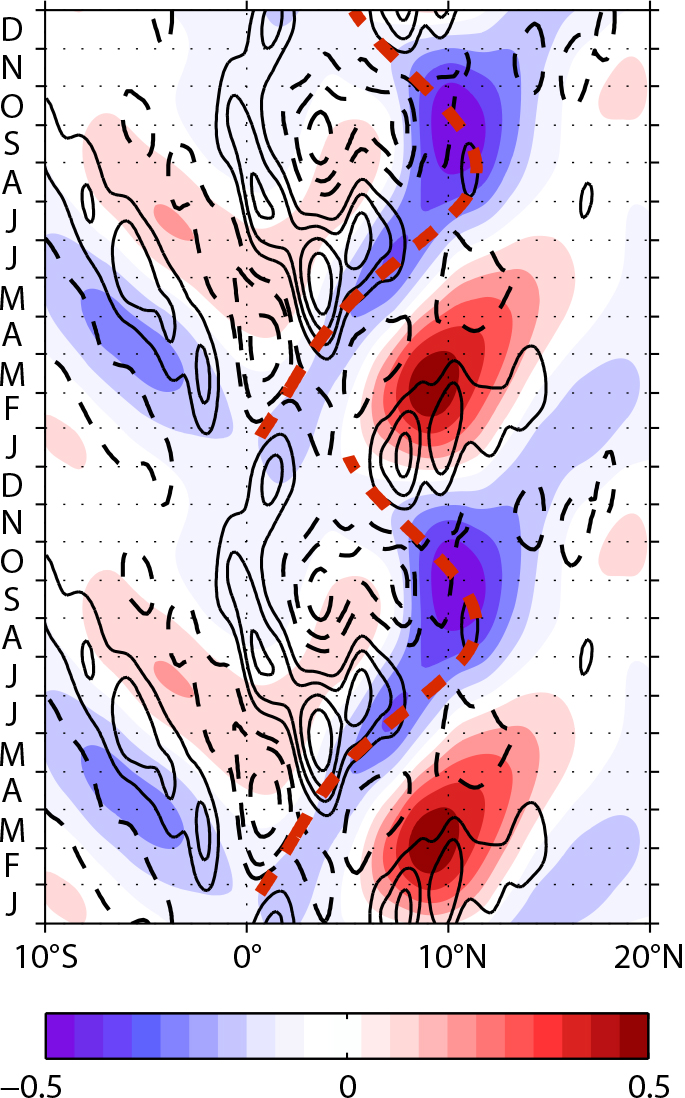
Figure 4. Latitude-time plot of the zonally averaged seasonal SSS anomaly between 135°W and 115°W. Contours show rate of change in SSS due to meridional advection. Seasonal anomalies in the meridional advection term (ν ∂S/∂y) were computed in the same manner as seasonal SSS anomalies. Solid contours = positive anomaly. Dashed contours = negative anomaly. Contour interval is 0.05 psu/month. Zero contour is omitted. The thick red dashed line shows seasonal migration of the Intertropical Convergence Zone. > High res figure

 

Interannual Variations

The strongest non-seasonal signal over the seven-year period of the satellite SSS time series is associated with the 2015–2016 El Niño event. To characterize spatial patterns of ENSO related SSS variability, Figure 5 shows the yearly mean SSS and SSS anomalies for each year from 2013 to 2017. The anomalies, except for year 2013, are computed relative to the 2013 mean, which represents a “neutral state” (Hasson et al., 2018). Averaging over a one-year period completely eliminates both the seasonal cycle and high-frequency variability, leaving only interannual variations.

 

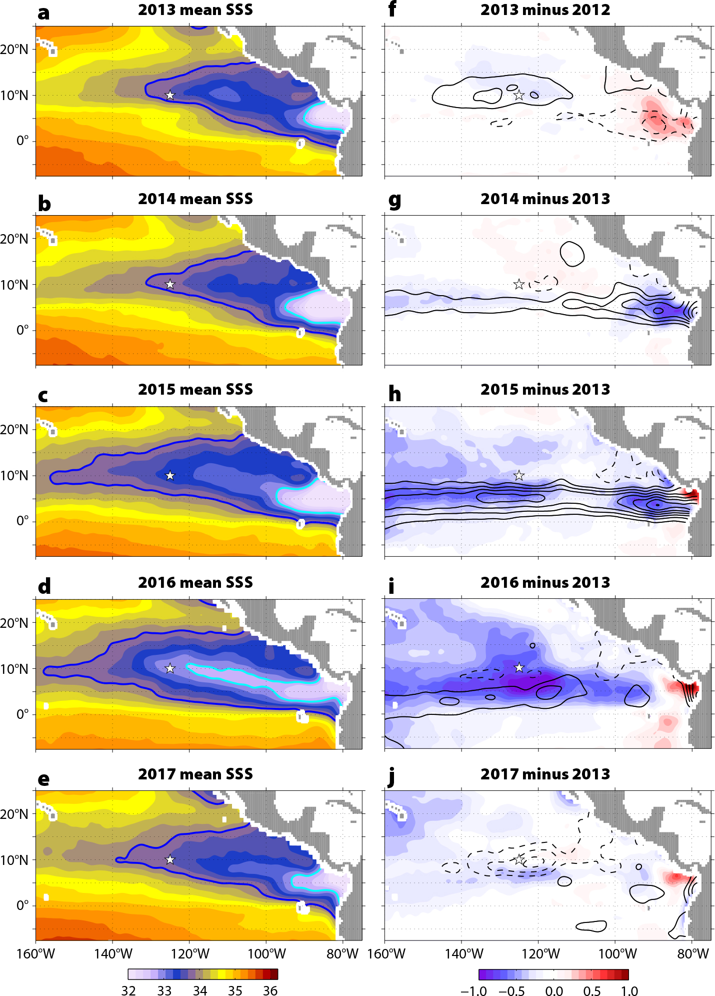
Figure 5. Yearly mean SSS fields for 2012 through 2017 (a–e) showing evolution during the El Niño event of 2015–2016. For each year the mean is computed from January through December. (f–j) The SSS anomalies for each year, 2014 through 2017, relative to the 2013 mean, except for panel (f), which shows the difference between the 2013 and 2012 means. Contours show S0(E – P)/h anomalies computed in the same manner as SSS anomalies. Solid contours indicate negative anomalies (rains more than normal), and dashed contours indicate positive anomalies (evaporates more than normal). Contour interval is 0.05 psu/month. Zero contour is omitted. > High res figure

 

There are significant differences in the size and geometry of the mean EPFP between the El Niño year and a normal year. The EPFP in 2016 is much larger and fresher than in, for example, 2013. In 2014 and 2015, negative SSS anomalies appear and grow in a zonal band between about 3°N and 8°N (Figure 5g,h), apparently reflecting the ENSO-related increase in precipitation that is typically centered along 5°N (Xie and Arkin, 1997; Delcroix, 1998), accompanied by the equatorward shift of the ITCZ (Tchilibou et al., 2015). The freshwater flux anomalies show anomalously rainy conditions in the same zonal band, supporting this inference. In the Gulf of Panama, the SSS anomaly is positive, presumably due to the lack of rainfall over land and the resulting decrease in river runoff (Fiedler and Talley, 2006).

In addition, significant freshening (>0.4 psu) is observed in 2015 around 20°N, south of the Hawaiian Islands (Figure 5h). Remarkably, this freshening is very persistent and can be observed even in 2017 (Figure 5j), while over the rest of the region, the ENSO-related negative SSS anomaly virtually vanished by this time. Hasson et al. (2018) argue that the freshwater anomalies around 20°N are specific to the 2015–2016 El Niño and are not part of the canonical SSS anomaly patterns typically associated with El Niño. They further hypothesize that the origin of these extra-equatorial anomalies is in the equatorial region to the west of the dateline and that horizontal advection, Ekman drift in particular, is the main driver of low SSS to the north of 10°N. However, this particular mechanism does not explain the remarkable persistence of the extra-equatorial freshwater anomalies; therefore, further study is needed.

Overall, the spatial patterns of SSS and precipitation anomalies are consistent with each other, with the surface freshwater forcing anomaly leading that of SSS by approximately one year. Yet, the SSS anomalies are slightly shifted northward relative to the maximum precipitation, by about 2°–3° of latitude, likely as a result of meridional Ekman advection (Delcroix, 1998; Tchilibou et al., 2015).

 

Intraseasonal Variations

Figure 2f shows that the intraseasonal patterns can be a dominant signal in the near-equatorial region. To see what comprises this signal, Figure 6a shows a time series of Aquarius/SMAP satellite SSS at 125°W, 1°N. Although intra­seasonal oscillations are apparent all along the time series, from about May 2016 to April 2017 (red dashed circle) there was a particularly strong signal, with a peak-to-peak change in SSS larger than 0.5 psu. This signal has a dominant period of about 30 days and can thus be attributed to the SSS signature of tropical instability waves (TIWs; Lee et al., 2012). Figure 6b shows the weekly SSS map centered on June 6, 2016. The spatial pattern of TIWs is clearly seen as cusp-like features between ~0° and 5°N with wavelengths of ~1,000 km (~10° of longitude). The waves propagate westward at a speed of ~0.5 m s^–1, as can be inferred from the Hovmöller diagram in Figure 6c,d. The diagram also shows that it is rather unusual for a strong SSS signal of TIWs to reach 125°W, as it did in 2016. This event is likely linked to the 2015–2016 El Niño, when significant freshening in the zonal band along ~5°N (Figure 5h) resulted in strong cross-equatorial SSS gradients. In other years, significant amplitudes of the SSS intraseasonal variability are observed in the eastern part of the basin, east of 110°W. The amplitudes, however, are strongly modulated by the seasonal cycle, with peak amplitudes during approximately the first half of the year, when the cross-equatorial SSS gradients in the eastern equatorial Pacific are stronger (not shown).

 

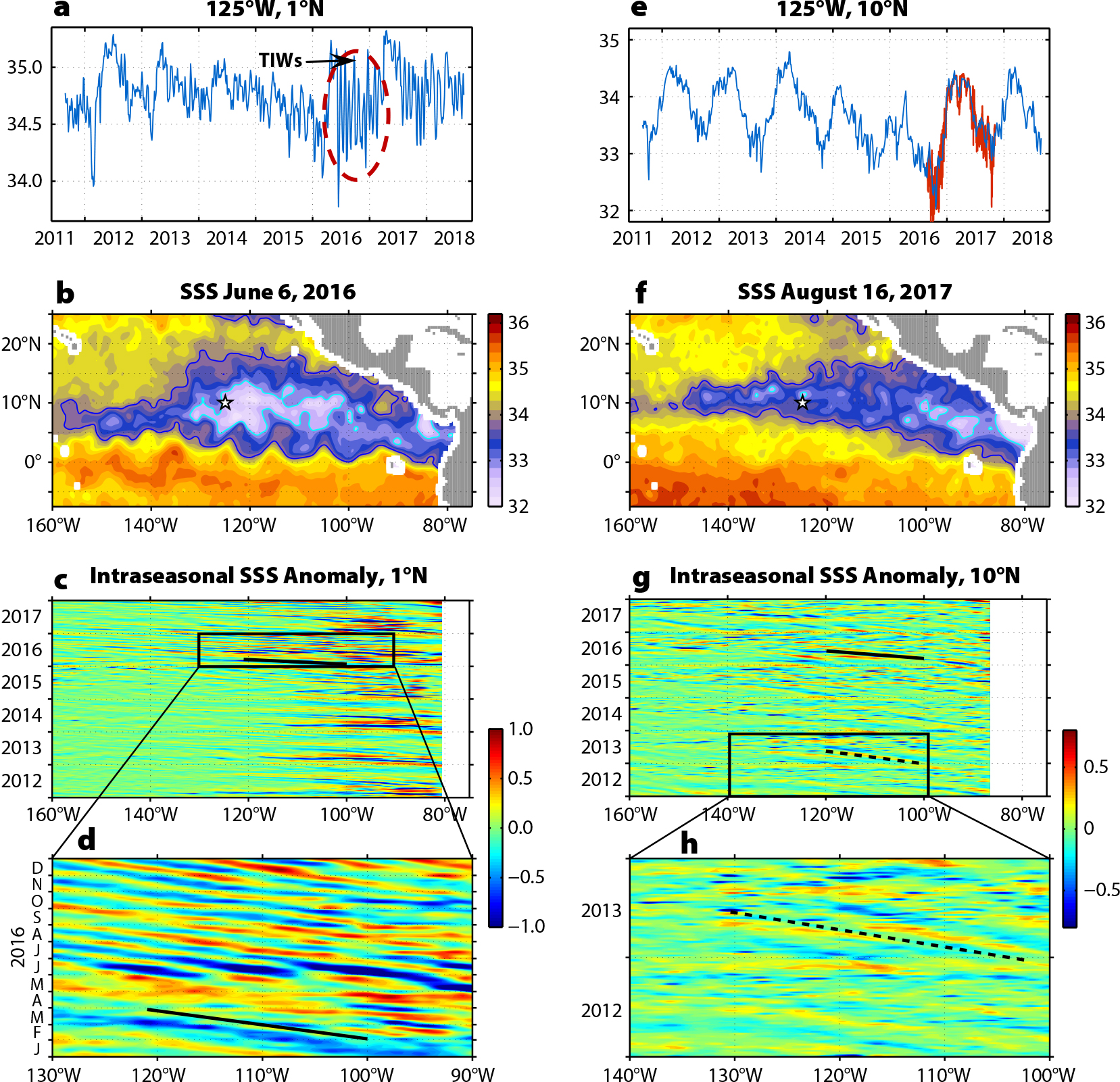
Figure 6. (a) Time series of SSS at 125°W, 1°N (white circle in Figure 2f) from Aquarius/SMAP satellite data. (b) Satellite SSS in the eastern tropical Pacific for the week centered on June 6, 2016. Tropical instability waves are observed between ~0° and 5°N as cusp-like features with wavelength ~1,000 km. (c) Longitude-time plot of intraseasonal SSS anomaly along 1°N. Propagating features are seen in the longitude-time plot as diagonal alignments of local maxima and minima. The solid line indicates a westward speed of 0.5 m s–1. (d) The same as in (c) but zoomed on the domain 130°–90°W, year 2016 (black rectangle in (c)). (e) Time series of SSS at 125°W, 10°N from Aquarius/SMAP satellite data (blue). The red line shows observations from the SPURS-2 central mooring at 1 m depth. (f) Satellite SSS in the eastern tropical Pacific for the week centered on August 16, 2017. (g) Longitude-time plot of intraseasonal SSS anomaly along 10°N. The solid (dashed) line indicates a westward speed of 0.3 (0.2) m s–1. (h) The same as in (g) but zoomed on the domain 140°–100°W, years 2012–2013 (black rectangle in (g)). > High res figure

 

At 10°N, a very different sort of intraseasonal SSS variability is observed. The time series of SSS at the location of the SPURS-2 central mooring (Figure 6e) illustrates the range of SSS variability, with the annual cycle dominating. Yet, short-scale variations are significant. The example weekly field in Figure 6f shows significant spatial variations in the central part of the domain where the SPURS-2 mooring sits right on the axis of a large freshwater pool elongated from east to west. The salinity distribution is very patchy in the pool, in part due to freshwater puddles likely caused by heavy rain events, and is measured in more detail as part of the SPURS-2 field campaign. The longitude-time plot of intraseasonal SSS anomalies along 10°N (Figure 6g) reveals the presence of westward-propagating features with phase speeds of ~0.2 m s^–1. The speeds are generally consistent with the average propagation speeds of large oceanic eddies in this latitude band reported by many studies (e.g., Chelton et al., 2011). The speeds are also remarkably consistent with the speeds of intraseasonal sea surface temperature (SST) and sea surface height (SSH) anomalies along this same latitude reported by Farrar and Weller (2006). Through extensive analysis of satellite and in situ data, Farrar and Weller conclude that the main source of intraseasonal variability in the region 9°–13°N in the eastern Pacific is baroclinic instability of the North Equatorial Current, which produces mesoscale eddies. The intraseasonal SSS signal at 10°N seems to be consistent with this hypothesis, as the majority of westward-propagating features observed in the longitude-time plot are formed locally; only very few can be traced to the eastern boundary. Locally, the SSS signal associated with the propagating features can reach 0.2 psu. Given this relatively large signal in SSS, eddies and the eddy-induced freshwater transport must play a significant role in the local freshwater balance (Delcroix et al., 2019). This still needs to be quantified and is the subject of an ongoing study.

 

SUMMARY AND CONCLUDING REMARKS

Observations of SSS by the Aquarius/SAC-D and SMAP satellite missions depict the eastern tropical Pacific Ocean as a highly variable and dynamic region, comprising variability over a broad range of temporal and spatial scales. In order to characterize dominant patterns of spatial and temporal variability of SSS in the region, the total SSS variance and the contributions of the seasonal, inter­annual, and intraseasonal components to it, as well as spatial patterns of each component of the variability, were computed from the seven-year time series of weekly satellite SSS data.

Maps of the SSS standard deviation and the fraction of variance show that the spatial patterns are quite different for each frequency band. The seasonal signal is highest along the core of the EPFP, along the coast of Central America, and in the Gulf of Panama. The interannual signal is high in a narrow zonal band along ~5°N. Intraseasonal variability is highest east of 110°W between 5°S and 10°N and in the Gulf of Panama. At the same time, the intraseasonal signal appears to be a dominant mode of variability in the zonally stretched near-equatorial region, most notably between 150°W and 90°W, accounting for more than 50% of the total SSS variance. The SPURS-2 site, at 10°N, 125°W, is located in the middle of a “pool” of high SSS variability (standard deviation greater than 0.5 psu), variability that is exhibited at many different temporal and spatial scales and, by inference, results from different processes.

On seasonal timescales, there seem to be two major centers of “action” producing the strong seasonal SSS anomalies with far-reaching consequences: one is along the equator and the other is along ~10°N. The anomalies propagate from there, presumably advected by ocean currents, westward-northwestward from 10°N and both southward and northward from the equator, and influencing regions far away from their generation sites.

On interannual timescales, the El Niño conditions of 2015–2016 dominate contributions to the interannual variance. During the El Niño event, fresher than average SSS appeared in a narrow zonal band between about 3°N and 8°N. These SSS changes appear to be in qualitative agreement with what would be expected if the changes were governed by ENSO-related changes in the surface freshwater flux term, whose spatial structure is determined to a large extent by precipitation. Yet, meridional offset between the SSS minimum and the surface freshwater flux maximum indicates a non-​negligible role of meridional Ekman advection. Likewise, north of about 10°N, changes in SSS cannot be explained by changes in freshwater forcing, indicating the dominant role of oceanic processes.

Intraseasonal SSS variance is greatest in the Gulf of Panama, although its contribution to the total SSS variance is greatest in a relatively narrow near-equatorial band between approximately 4°S–4°N and 150°W–90°W. This is largely associated with the SSS signal of TIWs. Satellite observations of SSS demonstrate that the SSS amplitudes associated with the TIWs are modulated strongly by the seasonal cycle and exhibit strong interannual variability, which may impact the long-term changes in the ocean circulation and the hydrological cycle (Lee et al., 2012).

The SPURS-2 site is affected by another kind of intraseasonal variability related to westward propagating eddies. Although relatively small compared to the seasonal and interannual variability, the SSS signature of mesoscale eddies along 10°N is significant (up to 0.2 psu), indicating that eddies and eddy variability can play a significant role in the freshwater balance in the eastern tropical Pacific (Delcroix et al., 2019). In this regard, freshwater transport by mesoscale eddies and TIWs is one of the many processes by which freshwater input by rain is transformed from shallow, patchy puddles of freshwater into the large-scale distribution of salinity in the eastern tropical Pacific as we observe it.

Finally, it is worth noting that a significant part of the SSS variability described in this paper would be missed or significantly attenuated if the analysis were conducted using data sets that have coarser temporal and spatial resolution (e.g., Argo-derived gridded products). The satellite SSS data were extremely useful in delineating details of the EPFP’s seasonal, interannual, and intraseasonal behavior, providing a descriptive framework for the SPURS-2 field experiment. The SPURS-2 site appears to be located at the crossroads of many different processes that shape the distribution of SSS in the eastern tropical Pacific and beyond. Combined with SPURS-2 results, satellite observations of SSS will provide new insights into the processes controlling SSS distribution and variability, and will improve our understanding of elements of the global water cycle.

Melnichenko, O., P. Hacker, F.M. Bingham, and T. Lee. 2019. Patterns of SSS variability in the eastern tropical Pacific: Intraseasonal to interannual timescales from seven years of NASA satellite data. Oceanography 32(2):20–29, https://doi.org/10.5670/oceanog.2019.208.

Alory, G., C. Maes, T. Delcroix, N. Reul, and S. Illig. 2012. Seasonal dynamics of sea surface salinity off Panama: The far Eastern Pacific Fresh Pool. Journal of Geophysical Research 117, C04028, https://doi.org/​10.1029/2011JC007802.

Bingham, F.M., G.R. Foltz, and M.J. McPhaden. 2010. Seasonal cycles of surface layer salinity in the Pacific Ocean. Ocean Science 6:775–787, https://doi.org/10.5194/os-6-775-2010.

Bingham, F.M., V. Tsontos, A. deSharon, C.J. Lauter, and L. Taylor. 2019. The SPURS-2 eastern tropical Pacific field campaign data collection. Oceanography 32(2):142–149, https://doi.org/​10.5670/oceanog.2019.222.

Chelton, D.B., M.G. Schlax, and R.M. Samelson. 2011. Global observations of nonlinear mesoscale eddies. Progress in Oceanography 91:167–216, https://doi.org/10.1016/j.pocean.2011.01.002.

Delcroix, T., and C. Henin. 1991. Seasonal and interannual variations of sea surface salinity in the tropical Pacific Ocean. Journal of Geophysical Research 96:22,135–22,150, https://doi.org/​10.1029/91JC02124.

Delcroix, T. 1998. Observed surface oceanic and atmospheric variability in the tropical Pacific at seasonal and ENSO timescales: A tentative overview. Journal of Geophysical Research 103:18,611–18,633, https://doi.org/​10.1029/98JC00814.

Delcroix, T., A. Chaigneau, D. Soviadan, J. Boutin, and C. Pegliasco. 2019. Eddy-induced salinity changes in the tropical Pacific. Journal of Geophysical Research 124:374–389, https://doi.org/​10.1029/​2018JC014394.

Farrar, J.T., and R.A. Weller. 2006. Intraseasonal variability near 10°N in the eastern tropical Pacific Ocean. Journal of Geophysical Research 111, C05015, https://doi.org/10.1029/2005JC002989.

Fiedler, P.C., and L.D. Talley. 2006. Hydrography in the eastern tropical Pacific: A review. Progress in Oceanography 69:143–180, https://doi.org/10.1016/​j.pocean.2006.03.008.

Gordon, A.L., C.F. Giulivi, J. Busecke, and F.M. Bingham. 2015. Differences among subtropical surface salinity patterns. Oceanography 28(1):32–39, https://doi.org/​10.5670/oceanog.2015.02.

Guimbard, S., N. Reul, B. Chapron, M. Umbert, and C. Maes. 2017. Seasonal and interannual variability of the Eastern Tropical Pacific Fresh Pool. Journal of Geophysical Research 122:1,749–1,771, https://doi.org/10.1002/2016JC012130.

Hasson, A., M. Puy, J. Boutin, E. Guilyardi, and R. Morrow. 2018. Northward pathway across the tropical North Pacific Ocean revealed by surface salinity: How do El Niño anomalies reach Hawaii? Journal of Geophysical Research 123:2,697–2,715, https://doi.org/10.1002/2017JC013423.

Huffman, G.J., D.T. Bolvin, and R.F. Adler. 2016. GPCP version 1.2 One-Degree Daily Precipitation Data Set. Research Data Archive at the National Center for Atmospheric Research, Computational and Information Systems Laboratory, https://doi.org/​10.5065/D6D50K46.

Kessler, W.S. 2006. The circulation in the eastern tropical Pacific: A review. Progress in Oceanography 69:181–217, https://doi.org/10.1016/​j.pocean.2006.03.009.

Lee, T., G. Lagerloef, M. Gierach, H.-Y. Kao, S. Yueh, and K. Dohan. 2012. Aquarius reveals salinity structure of tropical instability waves. Geophysical Research Letters 39, L12610, https://doi.org/​10.1029/​2012GL052232.

Lindstrom, E., F. Bryan, and R. Schmitt. 2015. SPURS: Salinity Processes in the Upper-ocean Regional Study—The North Atlantic Experiment. Oceanography 28(1):14–19, https://doi.org/10.5670/oceanog.2015.01.

Maes, C., N. Reul, D. Behringer, and T. O’Kane. 2014. The salinity signature of the equatorial Pacific cold tongue as revealed by the satellite SMOS mission. Geoscience Letters 1:17, https://doi.org/10.1186/s40562-014-0017-5.

McPhaden, M.J., S.E. Zebiak, and M.H. Glantz. 2006. ENSO as an integrating concept in Earth science. Science 314:1,740–1,745, https://doi.org/10.1126/science.1132588.

Melnichenko, O., P. Hacker, N. Maximenko, G. Lagerloef, and J. Potemra. 2016. Optimum interpolation analysis of Aquarius sea surface salinity. Journal of Geophysical Research 121:602–616, https://doi.org/10.1002/2015JC011343.

Melnichenko, O., P. Hacker, T. Meissner, F. Wentz, and J. Potemra. 2018. Building a consistent multi-satellite SSS data record: A case study in the eastern tropical Pacific (SPURS-2). Paper presented at the 2018 Ocean Salinity Science Team and Salinity Continuity Processing Meeting, August 27–29, 2018, Santa Rosa, CA, https://salinity.oceansciences.org/docs/ossc2018_melnichenko_b.pdf.

SPURS-2 Planning Group. 2015. From salty to fresh—Salinity Processes in the Upper-ocean Regional Study-2 (SPURS-2): Diagnosing the physics of a rainfall-dominated salinity minimum. Oceanography 28(1):150–159, https://doi.org/10.5670/oceanog.2015.15.

Tchilibou, M., T. Delcroix, G. Alory, S. Arnault, and G. Reverdin. 2015. Variations of the tropical Atlantic and Pacific SSS minimum zones and their relations to the ITCZ and SPCZ rain bands (1979–2009). Journal of Geophysical Research 120:5,090–5,100, https://doi.org/10.1002/2015JC010836.

US CLIVAR Office. 2007. Report of the US CLIVAR Salinity Working Group. US CLIVAR Report 2007-1, Washington, DC, 46 pp., https://usclivar.org/sites/default/files/Salinity_final_report.pdf.

Yu, L., and R.A. Weller. 2007. Objectively analyzed air-sea heat fluxes for the global ice-free oceans (1981–2005). Bulletin of the American Meteorological Society 88:527–529, https://doi.org/​10.1175/BAMS-88-4-527.

Yu, L. 2014. Coherent evidence from Aquarius and Argo for the existence of a shallow low-​salinity convergent zone beneath the Pacific ITCZ. Journal of Geophysical Research 119:7,625–7,644, https://doi.org/​10.1002/2014JC010030.

Xie, S.-P., and P. Arkin. 1996. Analysis of global monthly precipitation using gauge observations, satellite estimates, and numerical model predictions. Journal of Climate 9:840–858, https://doi.org/10.1175/1520-0442(1996)009​<0840:AOGMPU>2.0.CO;2.

This is an open access article made available under the terms of the Creative Commons Attribution 4.0 International License (https://creativecommons.org/licenses/by/4.0/), which permits use, sharing, adaptation, distribution, and reproduction in any medium or format as long as users cite the materials appropriately, provide a link to the Creative Commons license, and indicate the changes that were made to the original content. Images, animations, videos, or other third-party material used in articles are included in the Creative Commons license unless indicated otherwise in a credit line to the material. If the material is not included in the article’s Creative Commons license, users will need to obtain permission directly from the license holder to reproduce the material.