INTRODUCTION
Surface waves are a familiar feature of the sea surface, but the ocean environment also exhibits an extensive array of other wave phenomena, including the more counterintuitive internal waves (IWs) that propagate within the ocean. Although these less-familiar waves may be difficult to conceptualize, they can simply be pictured as analogous to surface waves (Alford et al., 2015) that, rather than propagating along the air-sea interface, use the ocean’s seasonal or permanent pycnocline as their waveguide (where the vertical gradient of density is maximum within the water column).
Unlike the smaller surface waves, IWs may span up to hundreds of kilometers in the horizontal and 200 meters in amplitude, and they may induce the largest vertical velocities in the ocean (of the order of 1 m s–1). These waves are perpetually generated in the ocean, either by the wind (Levine, 2002; Guthrie et al., 2013) or by tides that oscillate over rough bottom topography (Jackson et al., 2012). In most cases, IWs can become highly nonlinear, steepening and disintegrating into isolated wave packets that consist of several internal solitons called internal solitary waves (ISWs; see Osborne and Burch, 1980).
ISWs may propagate over basin-scale distances and are now acknowledged to have a turbulent character in both their propagation and their dissipation stages (van Haren and Gostiaux, 2012; Smyth and Moum, 2012). They are considered a dominant energy source for vertical motion and diapycnal (i.e., across isopycnals) turbulent mixing characteristics that affect the dynamics of a variety of ocean processes (Garwood et al., 2020). ISWs have been studied for more than 100 years and constitute a classical subject in ocean sciences (see e.g., Grimshaw, 2002, and references therein). However, observing them in nature is often a challenge, and dedicated in situ measurements are costly and troublesome. Therefore, ISW research increasingly relies on satellite remote sensing, which allows quasi-continuous monitoring on a global scale (Jackson et al., 2012; da Silva et al., 2015).
How is it possible that waves propagating deep down in the water column can be observed from orbiting satellites? The answer is that surface currents associated with ISWs interact with surface waves, which results in unique signatures in sea surface roughness that can be detected by satellite sensors. In particular, synthetic aperture radars (SARs) that image the sea surface at oblique incidence angles (see Box 1) have been widely used to study ISW signatures at the sea surface for more than 40 years, and a series of theories has emerged since then to explain some features of their observed radar signatures (Alpers, 1985; Thompson, 1988; Romeiser and Alpers, 1997).
However, the details of the SAR imaging mechanism for ISWs, which is based on modulation of sea surface roughness, are still not fully understood. In particular, conventional theories cannot explain the exceptionally large radar signatures caused by large-scale ISWs associated with breaking surface waves. Furthermore, sea surface manifestations of ISWs have also been detected recently in the high-resolution radar altimeter data from the European Sentinel-3 satellite, called SAR radar altimeter (SRAL), which achieves high spatial resolution in the along-track direction of the satellite by using the SAR processing technique (Santos-Ferreira et al., 2018, 2019; Zhang et al., 2020). However, the effects of enhanced surface wave breaking on SRAL backscattered signals are undocumented.
This paper aims to investigate how ISW-induced surface wave breaking affects the backscattered signals of spaceborne SARs and SAR altimeters and how it contributes to the imaging mechanisms used to interpret a series of sea surface ocean processes in radar remote sensing of the sea surface.
BOX 1 | Satellite Radar Sensing of the Sea Surface
Two fundamentally different radar sensors operate from orbiting satellites: synthetic aperture radars that emit radar pulses at oblique incidence angles (typically between 20° and 60°) and generate radar images of the sea surface, and radar altimeters (RAs) that emit radar pulses at a nadir incidence angle (vertically) and measure sea surface properties in a narrow band along the satellite path. Both emit microwave pulses and record the subsequent echoes. However, the scattering mechanisms that determine the intensities and shapes of the backscattered radar pulses are intrinsically different, and they survey different aspects of ocean dynamics (see Figure B1-1 for an ISW). Radar backscattering from the sea surface at oblique incidence angles in SARs is dominated by Bragg scattering, while radar backscattering at nadir incidence angles in RAs is dominated by specular reflection (Valenzuela, 1978). An important difference between these two scattering mechanisms is that, for specular reflection in RAs, the backscattered radar intensity decreases with increasing sea surface roughness, whereas it increases for Bragg scattering in SARs (see Figure 2 in Magalhaes and da Silva, 2017).
SARs acquire high-resolution images (up to the order of 1 m) of the ocean’s surface. The backscattered radiation returned to the satellite can be described, to first order, by Bragg scattering theory, which accounts mostly for radar backscattering from small-scale waves with wavelengths of the order of centimeters to decimeters (Valenzuela et al., 1978; Ager, 2013). In contrast to SARs, RAs are not imaging sensors; their echoes are recorded along a one-dimensional satellite ground track (usually referred to as along-track data). Nominal spatial resolution of conventional RAs in the along-track and cross-track directions is of the order of 10 km, while the resolution of new types of RAs, called SAR altimeters, is of the order of a few hundred meters in the along-track direction (for more details see Santos-Ferreira et al., 2018, and references therein).
These radar-satellite sensors use microwaves as their sensing radiation with wavelengths of the order of centimeters (e.g., X- and C- bands have typical wavelengths of 3 cm and 6 cm, respectively), and to leading order they sense the roughness of the sea surface at scales comparable to their emitted electromagnetic radiation. In general, however, the ocean surface also contains longer-scale waves, which evolve when moderate to strong winds blow over the sea surface for a sufficiently long time (resulting from wave-wave interaction in which energy is transferred from short-scale waves to longer-scale waves). These longer waves eventually break and form whitecaps on the sea surface, but their contributions to radar backscatter are not yet understood or even accounted for.
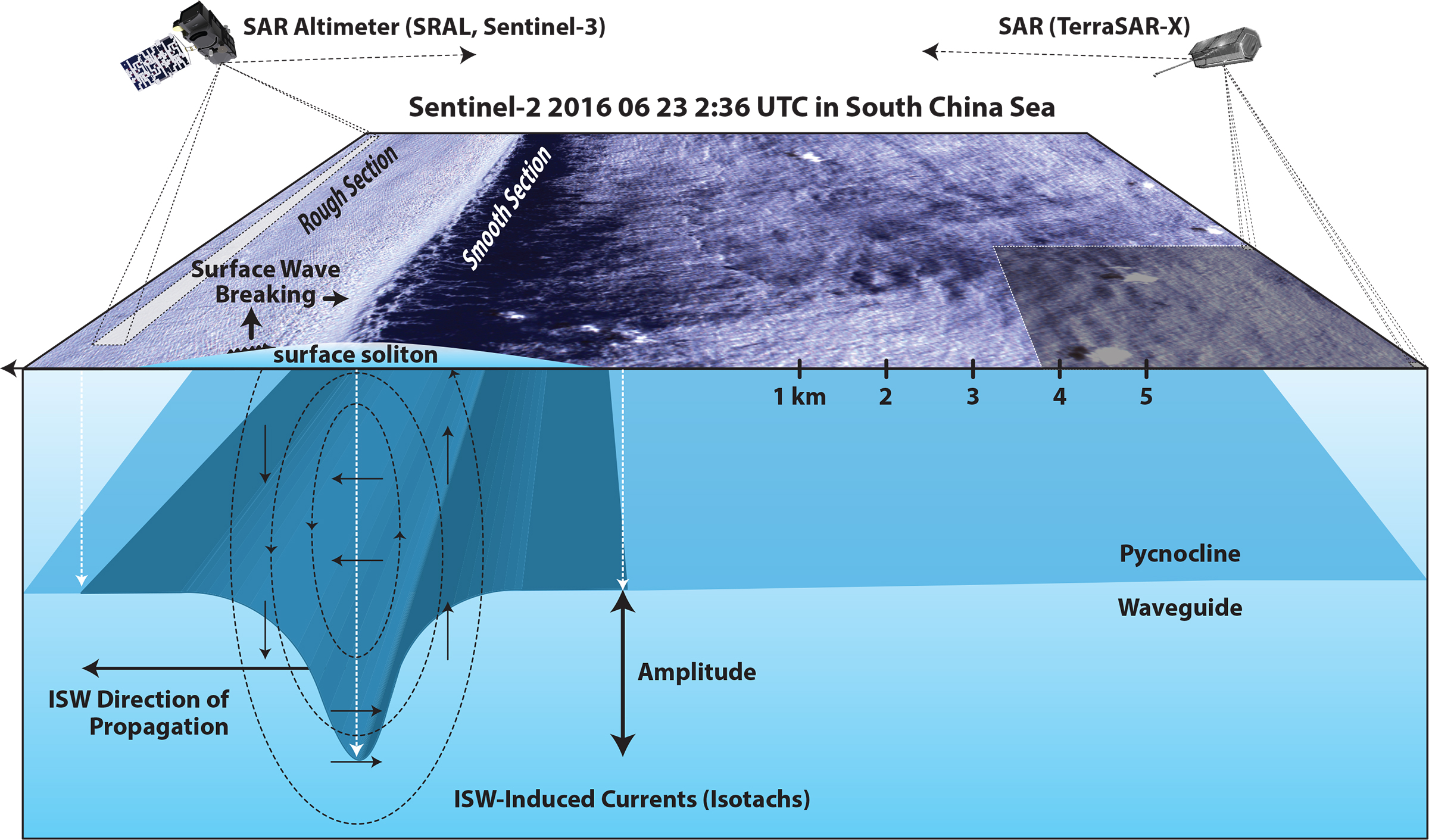
Figure B1-1. Schematic drawing illustrating how an ISW in the interior of the ocean is imaged by a nadir-looking SAR altimeter and a side-looking SAR (ground footprints not to scale). The ISW propagates along the pycnocline and generates convergence and divergence in surface currents, which modulate the sea surface roughness. An optical image acquired by the Multispectral Instrument (MSI) onboard the Sentinel-2 satellite shows on the left-hand side a sea surface signature of an ISW consisting of a rough section and a smooth section. Evidence of wave breaking is seen in the leading rough section (whitecaps), Note that maximum sea surface roughness is not located above the deepest depression of the pycnocline associated with the ISW, but in front of it, as predicted by theory (Alpers, 1985) and observed (Plant et al., 2010). > High res figure
|
SURFACE WAVE BREAKING INDUCED BY STRONG ISWs
Surface wave breaking (often seen as whitecaps on the sea surface) is a ubiquitous phenomenon in the ocean, especially at medium to high wind speeds. However, surface waves can also break in the absence of wind, for instance, when swell shoals on a beach. This paper deals with surface wave breaking that is not generated by the action of the wind but rather by interaction with an ISW, and how its sea surface signatures affect radar-based sensors onboard satellites.
There are countless observations of elongated bands of choppy waters associated with enhanced surface wave breaking. An early observation of this phenomenon in the Andaman Sea described by Maury (1861) was later identified as sea surface manifestations of large-scale ISWs (Perry and Schimke, 1965; Osborne and Burch, 1980). In particular, Osborne and Burch (1980) reported from their work in the Andaman Sea that these bands of choppy water contained short, steep, randomly oriented surface waves that stood out distinctly in an otherwise calm sea (hinting at low winds), which they attributed to sea surface manifestations of ISWs. Furthermore, these authors found that sea surface manifestations of ISWs had distinct surface roughness bands with breaking waves 1.8 m high, after which wave height quickly dropped to less than 0.1 m so that the ocean surface had the appearance of a millpond—and the entire process repeated as individual solitons passed beneath the ship.
Similar descriptions have been reported in other studies, and enhanced surface wave breaking associated with large-scale ISWs is now widely accepted. For example, Figure 1 shows sea surface manifestations of a strong ISW containing surface wave breaking, which appears to have wavelengths of the order of meters. Likewise, large-scale ISWs with enhanced surface wave breaking may be equally imaged in high spatial resolution satellite images (see online Figure S1).
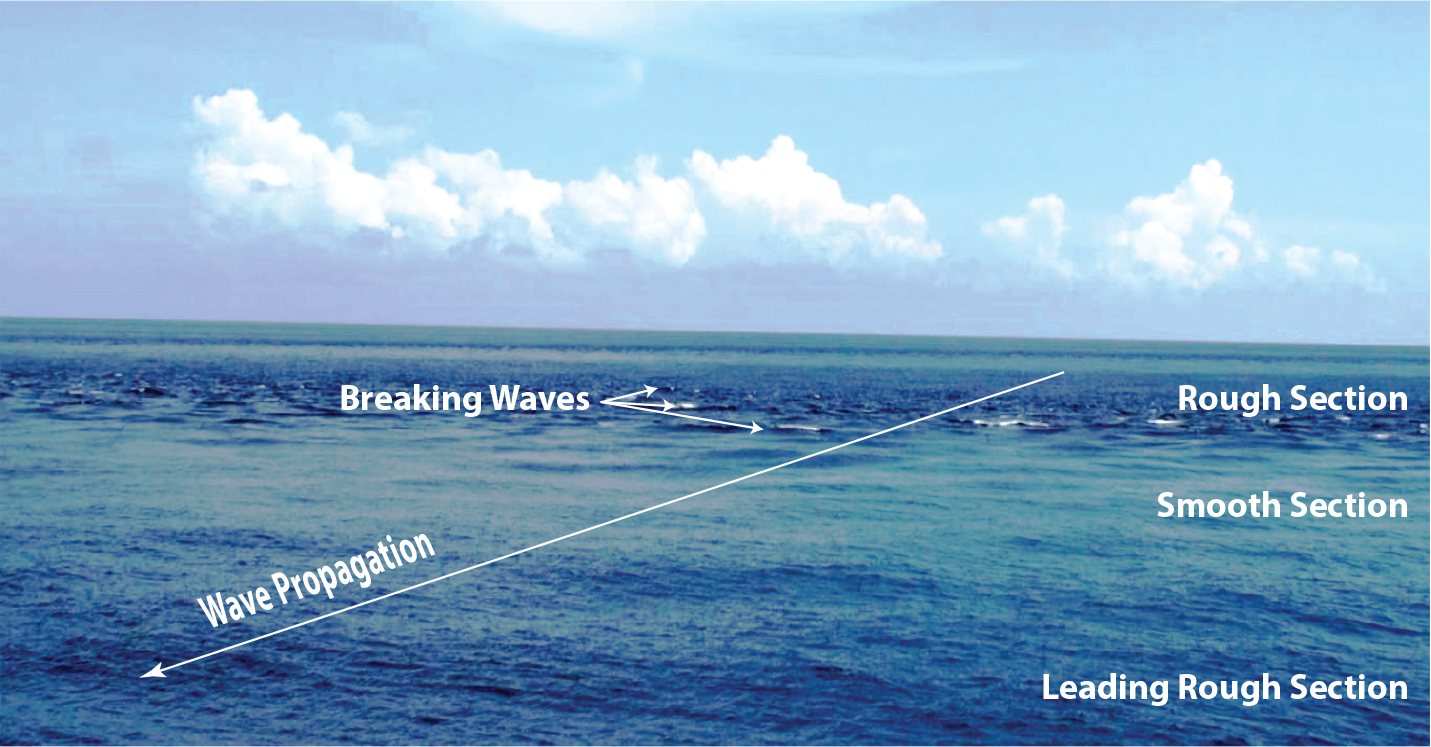
Figure 1. Photograph taken from a ship in the South China Sea on April 27, 2008, showing sea surface signatures of internal solitary waves (ISWs). A section of enhanced sea surface roughness is seen up front, followed by a reduced (smooth) sea surface roughness that in turn is followed by enhanced sea surface roughness containing evidence of surface wave breaking (i.e., whitecaps). Courtesy of Guozhen Zha. > High res figure
|
The increase in surface wave height in the roughness bands associated with ISWs has been extensively investigated. In particular, resonant interactions between surface waves and ISWs have been studied theoretically by Phillips (1973, 1977), Lewis et al. (1974), and Craig et al. (2012) and verified in the laboratory by Lewis et al. (1974) and Kodaira et al. (2016). Resonance occurs when the group velocity of the surface waves matches the phase speed of the IWs. Fueled by continuous input of energy from an ISW, resonant surface waves grow until they are dissipated by wave breaking or energy transfer to shorter waves via nonlinear hydrodynamic interaction. Lyzenga (2010) found that the energy transfer mechanism, in particular at X-band, also leads to larger modulation depths (or image contrasts) than predicted by previous SAR imaging theories regarding ISWs. However, we conjecture that wave breaking dominates dissipation of resonant waves and that scattering from breaking waves is the dominant contributor to the mechanism that results in large ISW radar signatures.
However, resonant interaction is not the only mechanism by which ISWs modify sea surface roughness. Surface waves of all wavelength scales interact with the varying surface current fields associated with ISWs to increase their amplitudes in the convergent sections of the surface current field, but not in the breaking of waves (Plant et al., 2010). This interaction can be modeled by weak hydrodynamic interaction theory (Alpers, 1985), which predicts a moderate increase in the amplitude of waves having wavelengths of the order of centimeters to decimeters in the roughness bands, but it does not predict an exponential growth of a single (resonant) wave that eventually breaks.
SURFACE WAVE BREAKING: CONTRIBUTIONS TO SAR IMAGING OF ISWs
The conventional theory of SAR imaging of ISWs employs weak hydrodynamic interaction and Bragg scattering (Alpers, 1985). This theory is successful in explaining SAR observations of ISWs with small modulations of the sea surface roughness (particularly at L-band) but fails to explain the often observed large modulation of the backscattered radar signal (particularly at X- and C-band). Similarly, advanced theories based on weak hydrodynamic interaction theory and the composite surface (or two-scale) Bragg model (Thompson, 1988; Brandt et al, 1999; Lyzenga, 2010) cannot fully explain the large modulations observed in X-band SAR images of ISWs (Thompson and Gasparovic, 1986). In these theories, radar backscattering from breaking surface waves is not included. However, it is now known that breaking surface waves play a key role in radar imaging of ISWs as first pointed out by Kudryavtsev et al. (2014). By analyzing C-band co-polarization (HH and VV) Radarsat-2 images, they showed that the radar backscattering from the sea surface roughness bands generated by ISWs often contain a non-polarized component (i.e., a non-Bragg component). They attribute it to the radar backscattering from breaking or nearly breaking surface waves with wavelengths of the order of meters and decameters. In this section, we describe carrying out a similar analysis using TerraSAR-X images, and we show that at X-band the radar signatures of ISWs contain a non-polarized component, which seems to be stronger than at C-band. Furthermore, our analysis of co- and cross-polarization (VV and VH) Sentinel-1 images of strong ISWs shows that breaking surface waves also exhibit a strong signal at cross-polarization that cannot be explained by two-scale Bragg scattering theory.
Co-polarized TerraSAR-X SAR Images
In this section, we present SAR images acquired by the German Earth-observation satellite TerraSAR-X (launched in 2007), which carries an X-band (9.65 Ghz) SAR. Figure 2a,b shows TerraSAR-X images acquired simultaneously at HH and VV polarizations over the western Mediterranean Sea. Both images show radar signatures of an eastward propagating ISW packet generated in the Strait of Gibraltar. At the time of the image acquisition, a light wind of about 3 m s–1 was blowing from the east.
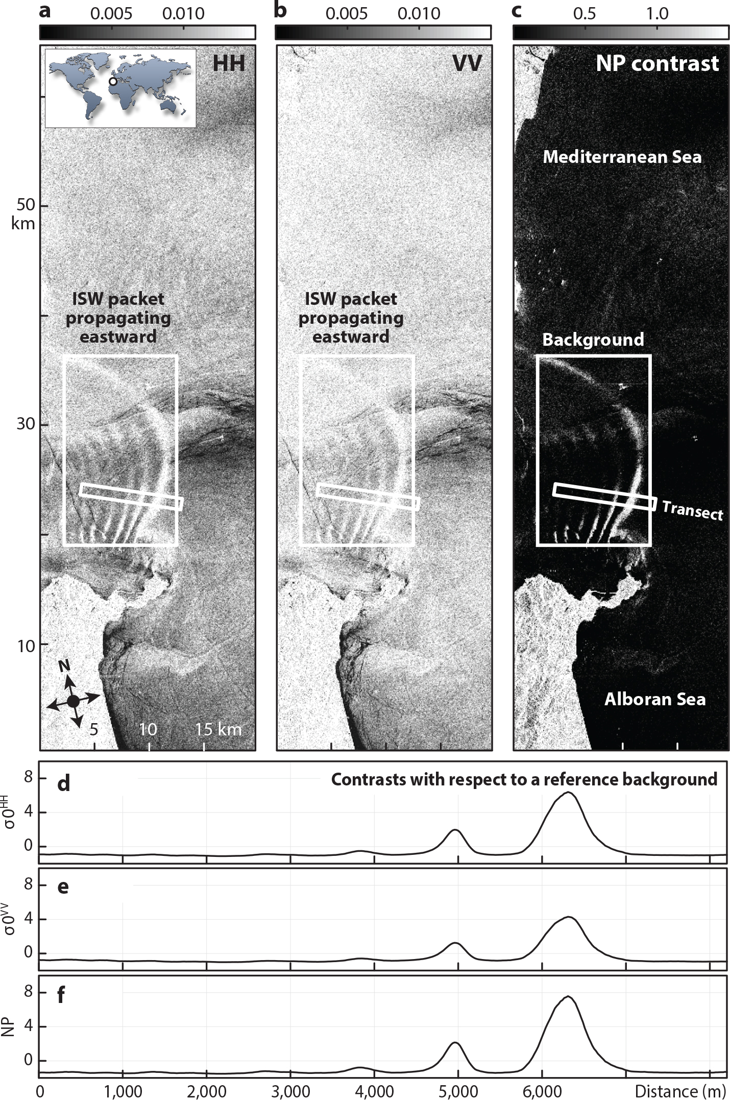
Figure 2. TerraSAR-X image (X-band in stripmap mode, spatial resolution of 6 m) acquired simultaneously at HH (a) and VV (b) polarizations (linear units) over the western Mediterranean Sea on August 17, 2009, at 06:29 UTC (see inset for location). The mean incidence angle is 31.5° and a wind of about 3 m s–1 was blowing from the east at the time of acquisition. (c) Image of the non-polarized (NP) contribution. (d) Profile showing the contrast in HH polarization along the (white) transect inserted in panel (a) (normalized by the mean value in the white rectangle). (e) Same as (d) for VV polarization. (f) Same as (d) for the non-polarized component. > High res figure
|
In order to investigate the physical mechanism causing the strong modulations visible in Figure 2a,b, we apply the same method to the TerraSAR-X data as Kudryavtsev et al. (2003, 2005, 2013, 2014) in their analysis of C-band Radarsat-2 data. These authors assume that the radar backscattering from the sea surface results from the superposition of two scattering mechanisms: a composite-surface Bragg scattering (B) and a non-polarized (NP) scattering. The co-polarized normalized radar cross section (NRCS or σ0, which is a measure of the power of the received radar backscatter) may be written as
σ0pp = σ0Bpp + σ0np, (1)
where the superscripts (pp) denote the polarizations of the transmitted and received radar signals (pp = HH or VV). Note that the first term in Equation 1 is polarization-dependent, whereas the second one (σ0np) is not. Dual co-polarization radar data (i.e., HH and VV as in Figure 2) allow comparison of the fraction of non-polarized scattering with the total radar backscattering as shown by Kudryavtsev et al. (2013). This is achieved by combining VV and HH images (σ0VV and σ0HH) in a polarization difference and a polarization ratio as follows:
Δσ0 = σ0VV – σ0HH = σ0BVV – σ0BHH, (2)
σ0HH / σ0VV = (σ0BHH + σ0np) / (σ0BVV +σ0np). (3)
Using Equations 1 to 3, we generate a σ0np image from the HH and VV images according to
σ0np = σ0VV – Δσ0 / (1 – PB), (4)
where PB = σ0BHH/ σ0BVV denotes the polarization ratio as given by the composite (or two-scale) Bragg scattering theory (see Valenzuela, 1978). In our case, PB = 0.39, which was computed for TerraSAR-X and for an incidence angle of 31.5°, and we recall that this ratio is independent of the shortwave spectrum, but dependent on the long waves via tilting effects.
The non-polarized contribution is shown in Figure 2c, where a reference background (mean σ0 values in the white squares) was used in the same way as in Kudryavtsev et al. (2014). The contrasts in NP contributions to the radar signature of the ISWs clearly stand out from the (darker) surrounding background—especially in the leading ISW and in the southern section of the wave packet.
To quantify the modulation depths in Figure 2 (i.e., the variation of NRCS relative to the background, δσ/σ0), the normalized contrast profiles of σ0BHH and σ0BVV along the ISW packets are shown in Figure 2d,e. These results reveal very large modulation depths up to 4 and 6 times the background backscatter power levels at VV and HH polarizations, respectively. These modulation depths are clearly too large to be explainable by conventional SAR imaging theories. Figure 2f shows even larger modulation depths close to 8 in non-polarized (NP) scattering, which suggests that the highest contrast is obtained when combining σ0HH and σ0VV images into a σ0np image according to Equation 4 (as shown in Figure 2c).
Co- and Cross-Polarization Sentinel-1 SAR Images
In this section, we present two C-band (5.4 GHz) SAR images acquired by the SARs onboard the European Sentinel-1A and 1B satellites (launched in 2014 and 2016) at VV and VH polarizations, which show radar signatures of large-scale ISWs. These examples were chosen to be representative of ISW radar images acquired during low and high winds (i.e., below 2 m s–1 and above 8 m s–1, respectively). We note that there is an issue with thermal noise in Sentinel-1 SAR images in the cross-polarization channels, which leads to a bias in NRCS values if uncorrected (Recchia et al., 2018). All results presented in this paper account for this issue.
Figure 3a,b shows two Sentinel-1B SAR images acquired simultaneously at VV and VH polarizations, with radar signatures of an ISW packet propagating eastward into the Mediterranean Sea under low wind conditions (<2 m s–1). Figure 3c shows the corresponding σ0VV and σ0VH profiles measured along the white arrows in Figure 3a,b (i.e., across the ISW pattern). The first soliton in the ISW packet has modulation depths of about 8 dB and 6 dB at VV and VH polarizations (respectively). The second wave has, as expected, smaller modulation depths, of about 5 dB at VV polarization and 1 dB at VH polarization, which we attribute to less breaking of the surface waves in its roughness section.
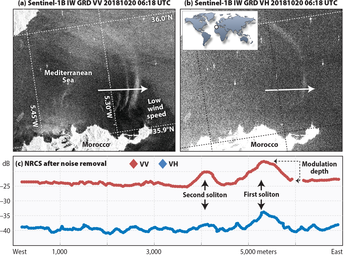
Figure 3. Sentinel-1B SAR image acquired at VV (a) and VH (b) polarizations on October 20, 2018, at 06:18 UTC showing ISW radar signatures in the Strait of Gibraltar (see inset for location). The image was acquired in the Interferometric Wide swath mode, with a 250 km swath and a spatial resolution of 5 m × 20 m (for Ground Range Detected products). Note that, in the darker area in the VV image (panel a), where the radar contrast of the ISW signature is strongest, the wind speed was probably less than 2 m s–1. (c) Normalized radar cross section (NRCS) profiles (in dB) along the white arrows in the images. The modulation depth for the first soliton is illustrated for reference. > High res figure
|
In Figure 4a,b, two Sentinel-1B SAR images acquired simultaneously at VV and VH polarizations under strong wind conditions (about 9 m s–1) depict radar signatures of an ISW packet propagating northwestward in the South China Sea. In this case, σ0VV and σ0VH profiles (Figure 4c) show a double-sign structure for the first and second solitons. The first wave shows modulation depths of about 3 dB at VV polarization and 4 dB at VH polarization, which decrease in the second soliton to about 1.5 dB and 2 dB.
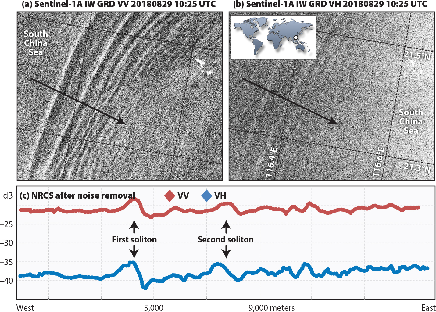
Figure 4. Same as Figure 3 for a Sentinel-1A SAR image acquired on August 29, 2018, at 10:25 UTC showing ISW radar signatures in the South China Sea (see inset for location). At the time of the SAR acquisition the wind was blowing at a speed of about 9 m s–1 from the south. (c) NRCS contrast profiles (in dB) along transects marked by black arrows in the images. > High res figure
|
When comparing the two cases, we can see that the modulation depths are smaller in high winds (Figure 4) than in light winds (Figure 3). Furthermore, Figures 3 and 4 suggest that ISW-induced modulation depths in the VH cross-polarization channel have values comparable with those in VV, and that VH modulation depths can even be stronger at high winds—meaning that in this case the ratio between VH and VV NRCS increases with wind speed.
Comparison of the NRCS profiles in Figures 3c and 4c also shows different structures in the sea surface (C-band) radar signatures of ISWs: Figure 3c shows an essentially single-sign structure of the ISW radar positive signature (i.e., only an increase of the NRCS relative to the background) for low winds speeds, while Figure 4 shows a double-sign structure. We attribute this to the difference in the wind speeds: in the first case (Figure 3), the wind speed was below the threshold for short wave generation (2 m s–1), and in the second case (Figure 4), the wind speed was high (9 m s–1) and wind-generated waves were present. These wind-generated waves are modulated by the ISW-induced surface currents. In particular, in the convergent sections, the amplitude of the short waves is increased, while in the divergent sections it is decreased, which results (according to Bragg scattering theory) in an increase and a decrease of the NRCS, respectively (and hence a double-sign radar signature). In contrast, in the case of low winds and the absence of short waves, the reduction of the NRCS in the divergent sections vanishes in the noise floor, such that only the convergent sections with enhanced NRCS values remain detectable, resulting in a single-sign radar signature of the ISW.
SURFACE WAVE BREAKING CONTRIBUTIONS TO RADAR ALTIMETER SIGNATURES OF ISWs
It is well established that internal tides (IWs of tidal period with horizontal length scales of hundreds of kilometers) can be successfully mapped from satellite by conventional satellite radar altimeters (Ray and Mitchum, 1996). Recently, Magalhaes and da Silva (2017) showed that the sea surface roughness signatures of large-scale ISWs with horizontal scales of the order of 10 km can also be detected by the conventional radar altimeter onboard the US/French Jason 2 satellite (launched in 2008). Santos-Ferreira et al. (2018, 2019) found that short-period internal solitary waves with horizontal scales of the order of 1 km can be detected by SAR altimeters due to their high resolution in the along-track direction (see Box 2). This new type of altimeter achieves high spatial resolution in the along-track direction by applying the SAR processing technique. Here, we build on the high along-track resolution of SAR altimeter data for measuring the normalized radar cross section and the significant wave height. These two parameters will be used in our analysis to investigate ISW-induced enhanced surface wave breaking. In this section, we analyze data acquired by the SAR radar altimeter (SRAL) in synergy with an optical image acquired by the Ocean and Land Color Instrument (OLCI). Both sensors fly on the same Sentinel-3A satellite (launched in 2016) and thus allow simultaneous measurements.
BOX 2 | Fundamentals of SAR Altimetry for ISW Detection
Satellite altimeters use nadir-pointed radar antennas that emit microwave pulses directly downward to “illuminate” the sea surface and record their subsequent echoes. The primary and most traditional measurement made by a satellite altimeter is the two-way travel time of the emitted pulse to the sea surface and back from radar echoes received from the backscatter radiation, which translates to distance after accounting for a series of corrections. However, the pulses that are reflected back to the altimeter are recorded onboard over a period of time, generating a “return waveform.” The waveform typically follows a well-known pattern that characterizes the sea surface roughness, from which geophysical information (SWH and NRCS) can be retrieved. Figure B2-1a provides an example for a conventional radar altimeter, in which the received power preceding the arrival of the return pulse is seen at the sensor’s (thermal) noise floor. The power of the return pulse rises rapidly and then decreases gently. As Brown (1977) and Rufenach and Alpers (1978) show, the SWH can be retrieved from the slope of the leading edge of the return pulse and the NRCS from the maximum power of the return pulse. Note that SWH is defined as four times the standard deviation of the surface elevations and relates closely to the older definition of SWH as the mean wave height (trough to crest) of the highest third of the waves. Thus, SWH estimates are a measure for large-scale sea surface roughness, and NRCS estimates are a measure for small-scale sea surface roughness.
New generation altimeters that use SAR processing to increase ground resolution are flying onboard ESA’s Sentinel-3 satellites and are usually termed SAR altimeters. However, SAR processing can only be used in the sensor’s direction of flight (i.e., in the along-track direction), meaning that ground resolution is sharpened to about 300 m in the along-track direction but retains the same broad resolution in the across-track direction as conventional altimeters (see Figure B2-1b). These sharpened ground resolutions are known to detect the sea surface signatures of ISWs more precisely than conventional altimeters. However, the return waveform in a SAR altimeter is more complex and needs special algorithms to retrieve SWH and NRCS. To this end, the SAR Altimetry MOde Studies and Applications (SAMOSA) model is used for describing the SRAL return wave form (Cotton et al., 2008; Boy et al. 2017); Figure B2-1a shows how its return waveform varies with different SWHs. The detection of ISWs by SAR altimeters depends on the angle between the flight direction and the propagation direction of the ISW. Optimal detection is achieved when this angle is zero. The larger this angle, the less sharp is the SAR altimeter signal (and it may even disappear). This is because the cross-track resolution is still very broad (as for conventional altimeters), and the return pulse may receive contributions simultaneously from ISW crests and troughs as illustrated below (see also discussions in Zhang et al., 2020). Because altimeters are active microwave sensors (like SARs), we expect they will also sense breaking surface waves, even though they sense the sea surface from different angles.
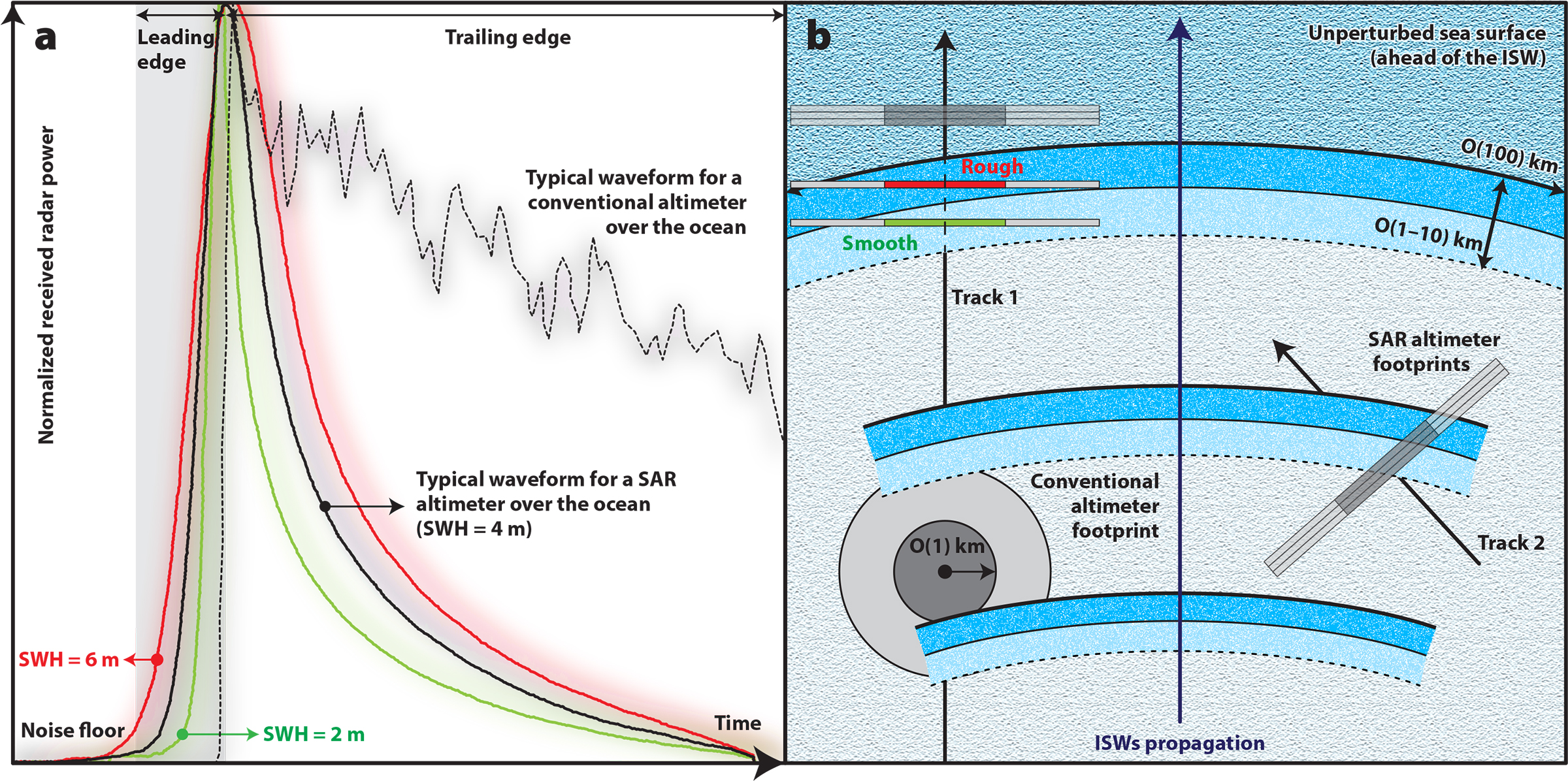
Figure B2-1. (a) Normalized SAR altimeter waveforms for an unperturbed sea surface (black) and with different SWHs. A waveform for a conventional altimeter is also shown as a dashed black line. (b) Schematic representation of an ISW packet and footprints of a conventional (circular shape) and a SAR altimeter (SRAL, rectangular shapes). Dark gray represents illuminated areas corresponding to maximum backscattered power, and light gray shows where power has decreased due to antenna effects. > High res figure
|
A Case Study Using Simultaneously Acquired Optical and SAR Altimeter Data from Sentinel-3A
Figure 5a shows a red-green-blue image composite from the OLCI (i.e., a quasi-true color image) acquired over the Brazilian shelf break, where a large-scale ISW with a characteristic width of about 10 km is seen propagating offshore in an almost meridional direction that is close to the along-track direction of the SRAL ground track. This means the increased ground resolution from the SRAL in the along-track direction (≈300 m) is favorably aligned to measure variations in sea surface properties (SWH and σ0) associated with ISWs and thus possible contributions arising from surface wave breaking.
Figure 5b,c shows how NRCS (σ0) and SWH vary when crossing the ISW pattern along the path marked by the white line (inserted in the black line, which denotes the ground track of the satellite) in Figure 5a. Figure 5b shows that σ0 decreases in the rough section of the ISW surface pattern by approximately 2.0 dB relative to the unperturbed background (ahead of the ISW and unaffected by it), while it increases only slightly in the wave’s trailing (smoother) section. We interpret this asymmetry between the rough and smooth sections as being related to an additional contribution from enhanced surface wave breaking in the front section of the ISW (similar to Figure 1).
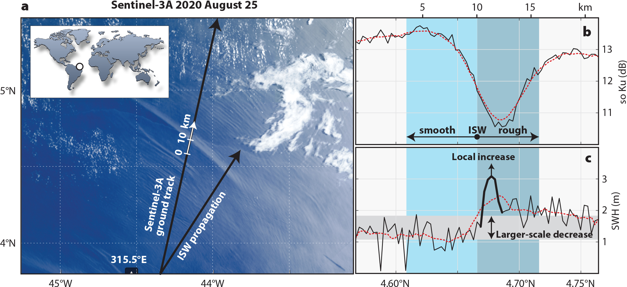
Figure 5. (a) Ocean and Land Color Instrument (OLCI) image acquired on August 25, 2020, at 11:22 UTC (see inset for location). The black arrows indicate the ground track of the satellite and the ISW direction of propagation. A distance scale (in white) highlights the large-scale ISW shown in the following panels. (b) Along-track co-polarized normalized radar cross section (Ku-band) measured by the synthetic aperture radar (SAR) altimeter (SRAL). (c) Same as (b) for significant wave height (SWH). A gray envelope highlights a decrease in SWH when comparing sections ahead and behind the ISW. Blue shades distinguish the ISW’s leading (rough) and trailing (smooth) sections. The red dashed lines are box moving averages (nine consecutive pulses). > High res figure
|
Figure 5c shows that SWH is higher in the leading section of the ISW pattern and lower in the trailing section, and that there is a sharp and localized “bump” of about 1m at the position of the roughness band of the ISW (as in Figure 4 in Santos-Ferreira et al., 2018). In contrast to the strong decrease of σ0 in this section due to reflection mainly from small-scale structures in the roughness band containing breaking waves (Figure 5b), the sharp increase in SWH is mainly due to the large-scale structures in the roughness band (i.e., to the higher waves). We recall that SWH is a statistical parameter of the wave field defined as the average wave height (measured from trough to crest) of the highest one-third of the waves. When a resonant wave grows beyond its maximum equilibrium point and breaks—due to energy transfer from the ISW propagating below—then a measurable increase in SWH is expected to appear in the altimeter’s SWH signature (to be further discussed in the next section).
Nine more cases were found with SWH profiles similar to those shown in Figure 5 (see online Supplement S2). As in Figure 5, these cases consistently show a decrease in SWH between the ISW’s leading and trailing sections of about 30% (on average) of the unperturbed SWHs (i.e., ahead of the ISW). These changes in SWH hold for different wind conditions and orientations and add to the robustness of the results presented in Figure 5.
SUMMARY AND DISCUSSION
In situ observations show that large-scale ISWs are often associated with breaking surface waves with wavelengths of the order of meters to decameters (i.e., intermediate-scale waves, see Figure 1). Here, we presented evidence that ISW-induced surface wave breaking leaves measurable (and distinct) signatures in SARs and SAR altimeter data that cannot be fully explained by present theories.
For SARs, we have documented in three distinct images exceptionally large increases in NRCS values associated with large-scale ISWs: one in a dual co-polarization (VV and HH) X-band TerraSAR-X SAR image (at low wind speeds; Figure 2), and two others in co- and cross-polarization (VV and VH) C-band Sentinel-1 SAR images (at low and high wind speeds; Figures 3 and 4). Our analysis of X-band TerraSAR-X data closely follows the method described in Kudryavtsev et al. (2014) that includes the addition of a non-polarized scattering mechanism (Kudryavtsev et al., 2003, 2005, 2013, 2014, 2019).
Kudryavtsev et al. (2014) found in their analysis of dual co-polarization C-band Radarsat-2 SAR images that the ISW pattern is best discernible (i.e., shows highest contrast) when the VV and HH polarization images (i.e., the σ0VV and σ0HH maps) are combined according to Equation 4 such that only the modulation caused by non-polarized scattering is retained. In their non-polarized images, the modulation depth (or image contrast) attains values up to 3 (their Figures 7 and 10), while in the HH image it attains only values up to 2. Our results from X-band SAR images (Figure 2) show modulation depths of up to 8 in non-polarized images, which suggests that the non-polarized scattering from surface wave breaking might be stronger at X-band than at C-band. We again reiterate that this exceptionally high contrast (observed at low wind speeds) cannot be explained by conventional radar backscattering theories involving the composite surface Bragg model (Thompson, 1988; Romeiser and Alpers, 1997; Brandt et al, 1999). As Thompson and Gasparovic (1986) show, the composite surface Bragg model cannot generate image contrasts larger than 1.5, and hence it greatly underestimates measured image contrasts (as in Figure 2).
Analysis of co- and cross-polarization (VV and VH) C-band Sentinel-1 SAR images shows that ISWs can give rise to NCRS increases of up to 6 dB (Figure 3). Such a large increase cannot be explained by Bragg scattering theory in conjunction with weak hydrodynamic interaction theory (Alpers, 1985). Although advanced scattering theories based on the composite surface Bragg model can generate some modulation at cross-polarization, they cannot account for the high modulation depth measured in the Sentinel-1 SAR images (≈6 dB), which we hypothesize to be associated with scattering from breaking waves. Evidently, non-polarization cannot account for cross-polarization scattering. These high values of radar backscatter at cross-polarization point to an additional scattering mechanism that must rely on some kind of polarized scattering. However, to date, there is no theory that can explain the high radar returns from breaking waves at cross-polarization, even though some speculations and hypotheses have been posed (see, e.g., Lee et al., 1996; Hwang et al., 2010; Voronovich and Zavorotny, 2011). Thus, modeling cross-polarization radar backscattering from the sea surface in the presence of wave breaking remains a challenging task for the future.
Analysis of high-resolution altimeter (SRAL) data acquired in synergy with optical data (OLCI) from Sentinel-3A shows that an ISW gives rise to a strong decrease in the NRCS (σ0) of the rough section of the ISW surface pattern of approximately 2.0 dB relative to the unperturbed background (ahead of the ISW), and a small increase in the trailing (smoother) section. Furthermore, the analysis reveals that the ISW imposes distinct signatures on the SWH signal that have not been documented previously (see Figure 5): (1) a sharp and localized increase in SWH in the leading and rougher section of the ISW pattern (over a distance of few kilometers), and (2) a drop in SWH from the leading section to the trailing section of the ISW pattern. Both effects have been detected in 10 different cases (see online Supplement S2) with varying imaging geometries and wind and wave conditions. We interpret the enhancement of the SWH at the location of the roughness band as being caused by breaking surface waves generated by hydrodynamic interaction of surface waves with the ISWs, and we interpret the difference in SWH in front of and behind the ISW pattern as being caused by energy dissipation due to surface wave breaking. Such decreases in SWH after the passage of an ISW have been observed in several other SRAL data sets (see online Supplement S2).
It should be noted that other scattering theories, which do not involve wave breaking, have been developed to explain the often observed large radar signatures of ISWs. The SAR imaging theories for ISWs of Thompson (1988), Lyzenga (2010), Craig et al. (2012), and Chen et al. (2017) all yield larger modulation depths than those predicted by the theory of Alpers (1985) and are thus closer to reality; but they all fail to predict the very large ISW radar signatures that are frequently observed. Thus, we conjecture that scattering from breaking waves must be included in a SAR imaging theory for ISWs. But such a theory presently does not exist, and its development remains a challenge for the future.
Acknowledgments
This work was funded by the EU and ESA, under subcontract CLS-ENV-BC-20-0017 “Multi Sensor Synergy Study for Sentinel-3C/D” between the University of Porto and Collecte Localisation Satellites, SA. Peter Meadows of BAE, UK, who is deeply involved in Sentinel-1 SAR calibration and processing, is appreciatively acknowledged. J.M. thanks the Portuguese funding agency Fundação para a Ciência e Tecnologia (FCT) under projects UIDB/04423/2020 and UIDP/04423/2020. A.M.S.-F. gratefully acknowledges FCT for PhD grant SFRH/BD/143443/2019. W.A. received support from the ESA/NRSCC Dragon 5 project. This work was funded by the Fundação para a Ciência e a Tecnologia under UIDB/04683/2020 project. We are very grateful to three reviewers and Oceanography Editor Ellen Kappel for suggestions and changes in style of this manuscript, which greatly improved its readability and the delivery of our message to a wider audience. This paper is dedicated to Ozíris de Lingen, for her beloved companionship.